3D landscapes and the Riemann sphere
All 3D rendering goes through PyVista. The matplotlib 3D backend was removed in 3.0, along with the capability flags that used to guard it — see the backend policy for the reasoning and the measurements behind making PyVista a required dependency.
Analytic landscapes
An analytic landscape lifts |f(z)| into height while keeping the phase colouring on the surface:
import complexplorer as cp

cp.plot_landscape_pv(
    cp.Rectangle(4, 4),
    lambda z: (z**2 - 1) / (z**2 + 1),
    cmap=cp.Phase(phase_sectors=6, auto_scale_r=True),
)
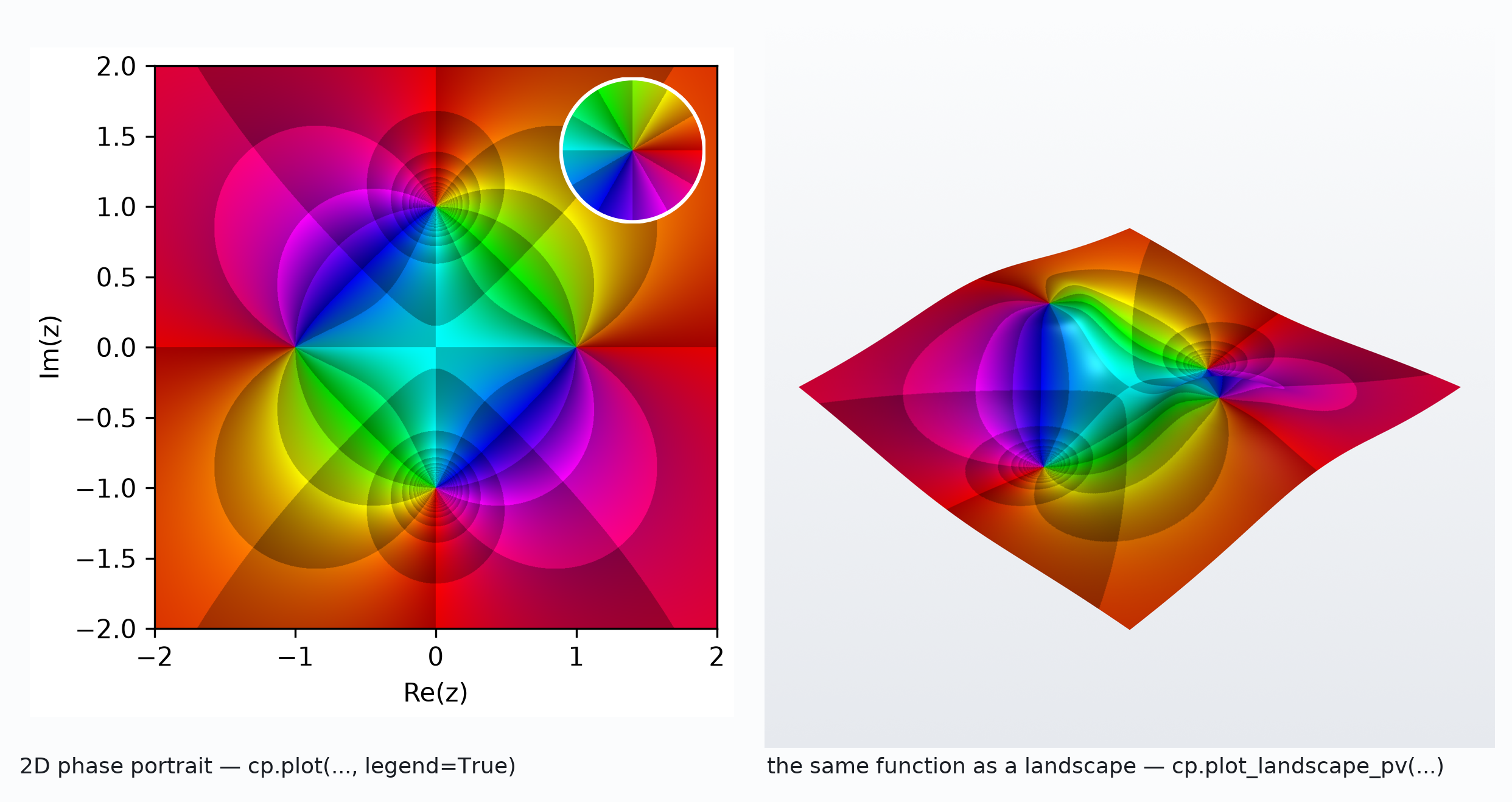
Zeros sink, poles rise, and the colours are unchanged from the flat portrait. pair_plot_landscape_pv
puts the domain and codomain side by side.
Modulus scaling
|f(z)| is unbounded near a pole, so something has to compress it before it becomes geometry.
That is what modulus scaling does, and it is the single most consequential setting in 3D:
The modes are constant, linear, linear_clamp, arctan, logarithmic, power, sigmoid,
adaptive, hybrid and custom. arctan is the safe default: it is smooth, bounded, and keeps a
pole from turning into an infinite spike. get_scaling_preset() bundles the settings the gallery
uses, such as "balanced" and "poles_emphasis".
If a relief looks like a forest of needles, the scaling mode is the dial to turn — not the resolution.
The Riemann sphere
Stereographic projection wraps the plane onto a sphere, so the point at infinity becomes an ordinary place you can look at:
The origin and infinity sit at opposite poles, and the unit circle becomes the equator. A function with a zero at the origin and a pole at infinity is, on the sphere, simply a function with a zero at one pole and a pole at the other — which is often the clearest way to see what it does.
Headless use and reproducible images
Every 3D renderer accepts filename and interactive=False, which writes an image instead of
opening a window. This is what scripts, CI and remote machines need:
cp.riemann_pv(
    lambda z: z / (z**10 - 1),
    resolution=200,
    modulus_mode="arctan",
    interactive=False,
    filename="relief.png",
    window_size=(1200, 1200),
    camera_position=(2.5, 2.5, 2.5),
)
Two things make the output reproducible rather than incidental:
- Set
camera_positionexplicitly. The default is a fixed tuple, but any interaction moves it; pinning it in the call is what makes two runs comparable. - Set
window_size. The image is rendered at that size, so it determines the resolution of what you get, independently of the samplingresolution.
On Linux without a display, set PYVISTA_OFF_SCREEN=true and run under a virtual framebuffer; the
project's own CI uses pyvista/setup-headless-display-action for exactly this.
return_plotter=True hands back the PyVista Plotter instead of rendering, so you can add
lighting, change the background or compose several meshes before writing the file. That is how
examples/showcase.py produces the images on this site.
Notebooks
PyVista's Jupyter backend uses trame, which has noticeably weaker antialiasing than a desktop
window. For figures you intend to keep, run the 3D renderers from a script rather than a notebook —
examples/scripts/ holds working examples.
Next
- Riemann surfaces — the multi-sheeted cover, which is a different object
- STL export — turning a relief into something printable