Gallery
Every image here is produced by examples/showcase.py from the curated preset registry
(cp.catalog) and the tour recipes in examples/tour.py. Thumbnails link to the
full-resolution render.
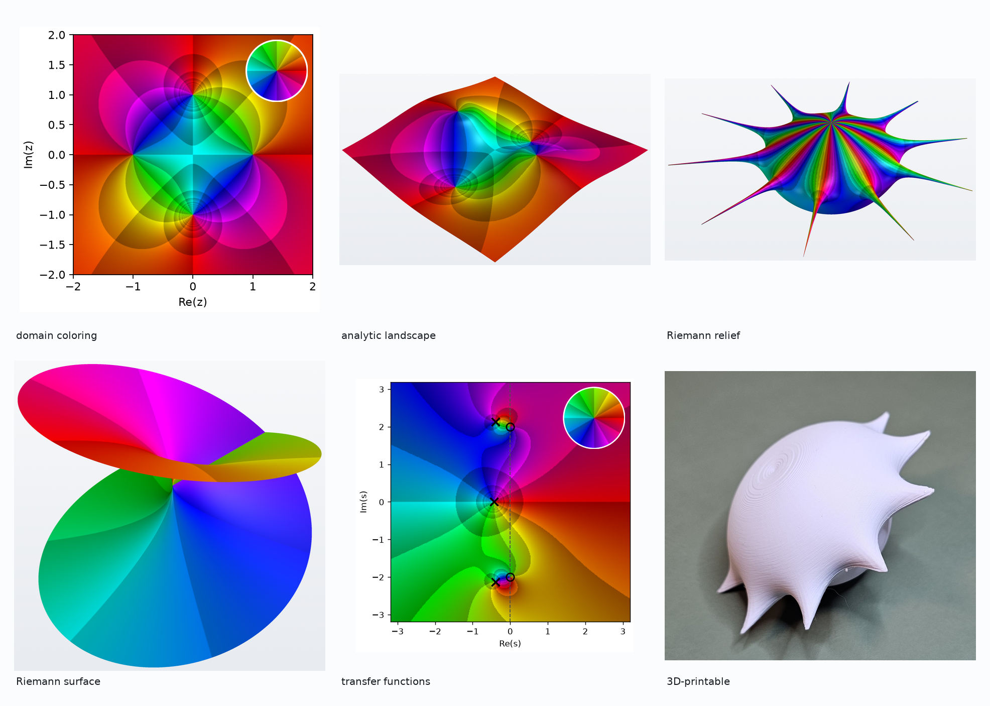
What is here
- Phase portraits — 8 figures
- Mapping and topology — 8 figures
- Riemann surfaces — 4 figures
- Engineering mode — 2 figures
- Colormaps — 17 figures
- Physical output — 9 figures
Phase portraits
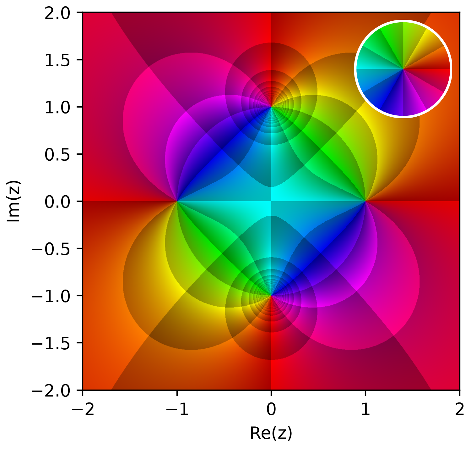
Hue is the phase of f(z); the shaded cells are contour bands of |f(z)|. Zeros and poles read as opposite winding directions.
Reading a phase portrait
Hue is the phase of f(z) and the shaded cells are its contour bands, so zeros and poles read as opposite winding directions. The inset legend is the same colormap applied to the identity map, which is what makes the picture decodable.
Show the code
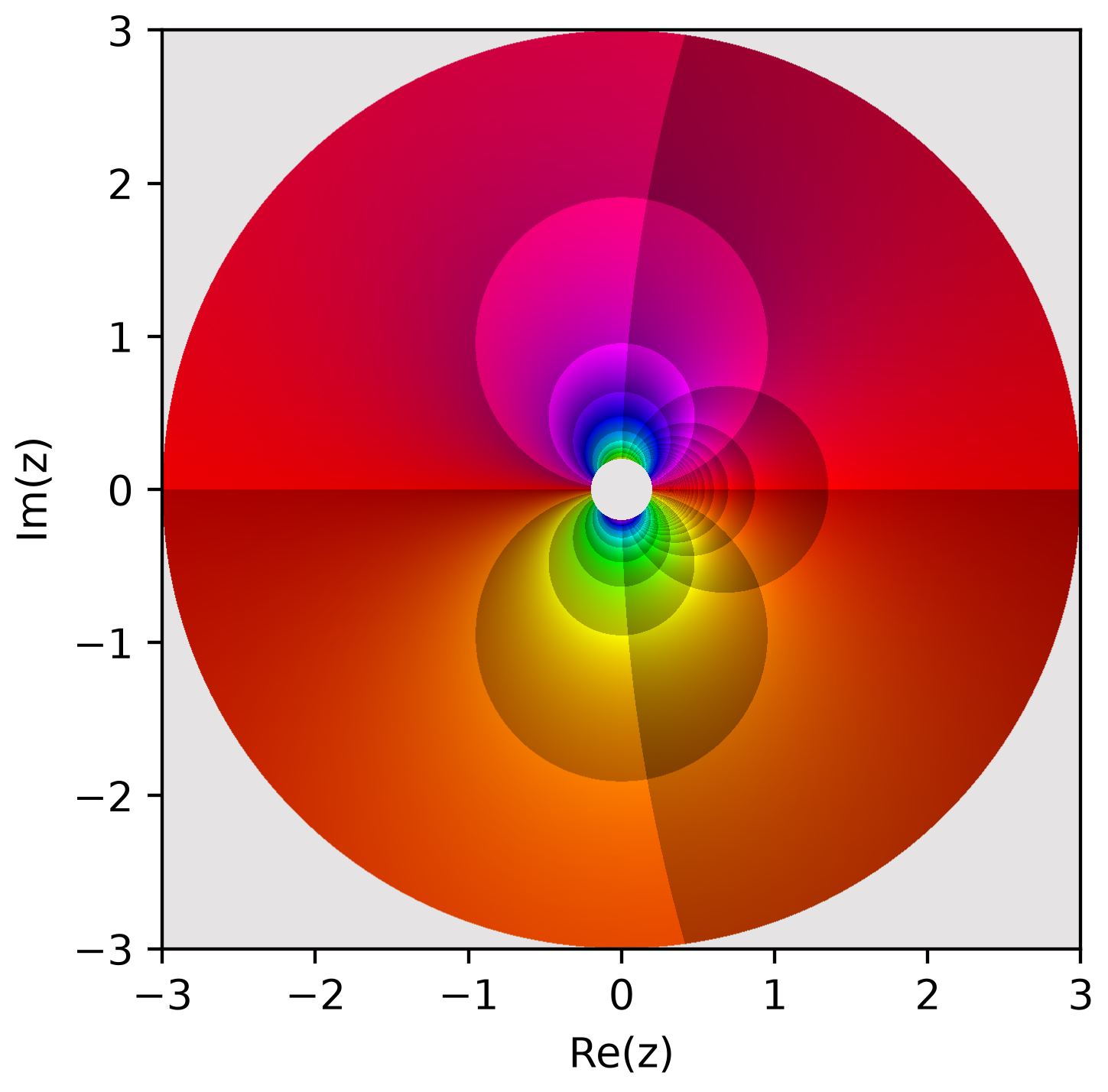
Essential singularity
exp(1/z) has an essential singularity at 0 — infinitely dense structure nearby.
Show the code
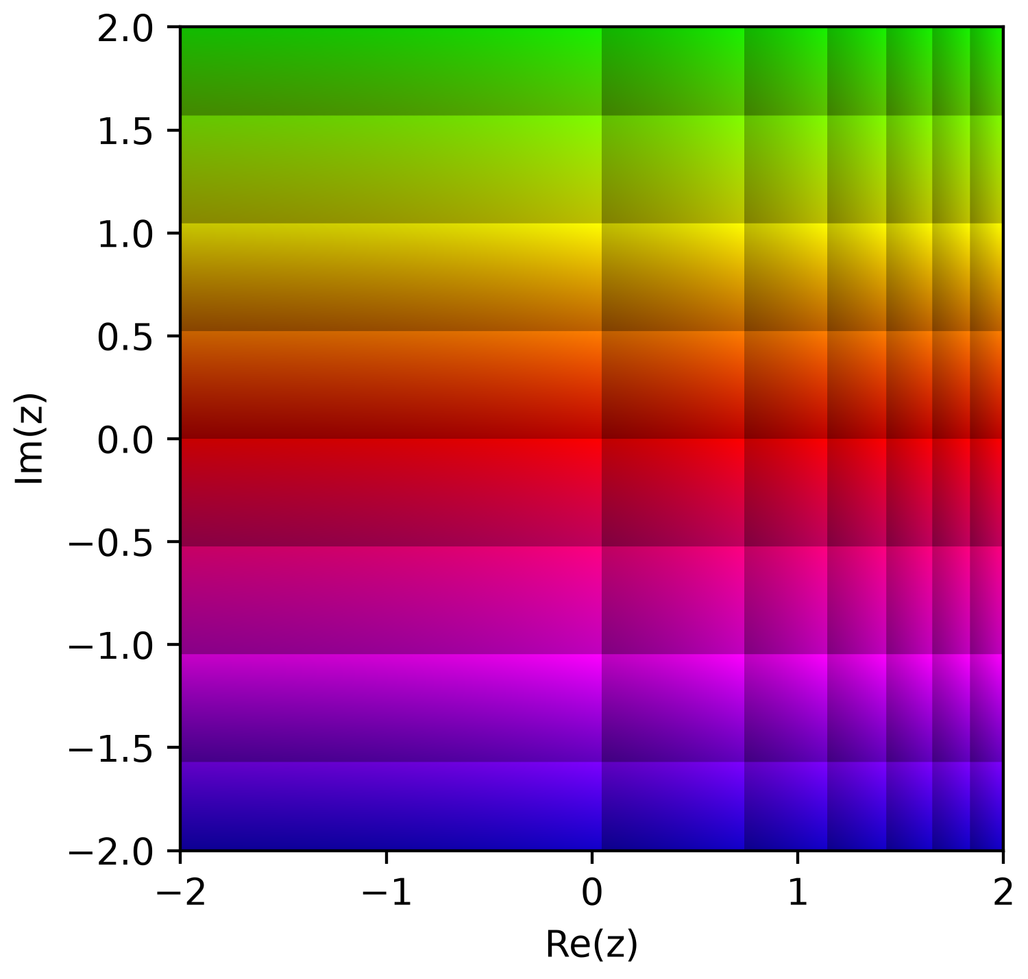
Exponential
Entire and never zero: no finite zeros or poles (an empty answer key).
Show the code
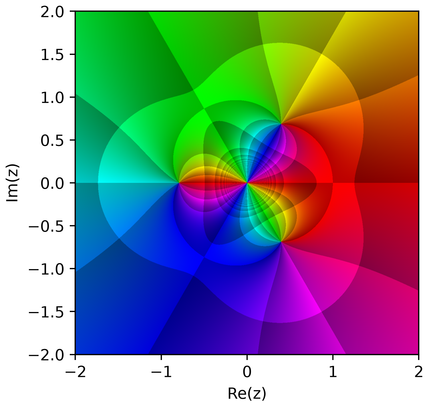
Newton map (z³ - 1)
The Newton iteration map for z³ - 1: an order-2 pole at 0 and three simple zeros at the cube roots of -1/2.
Show the code
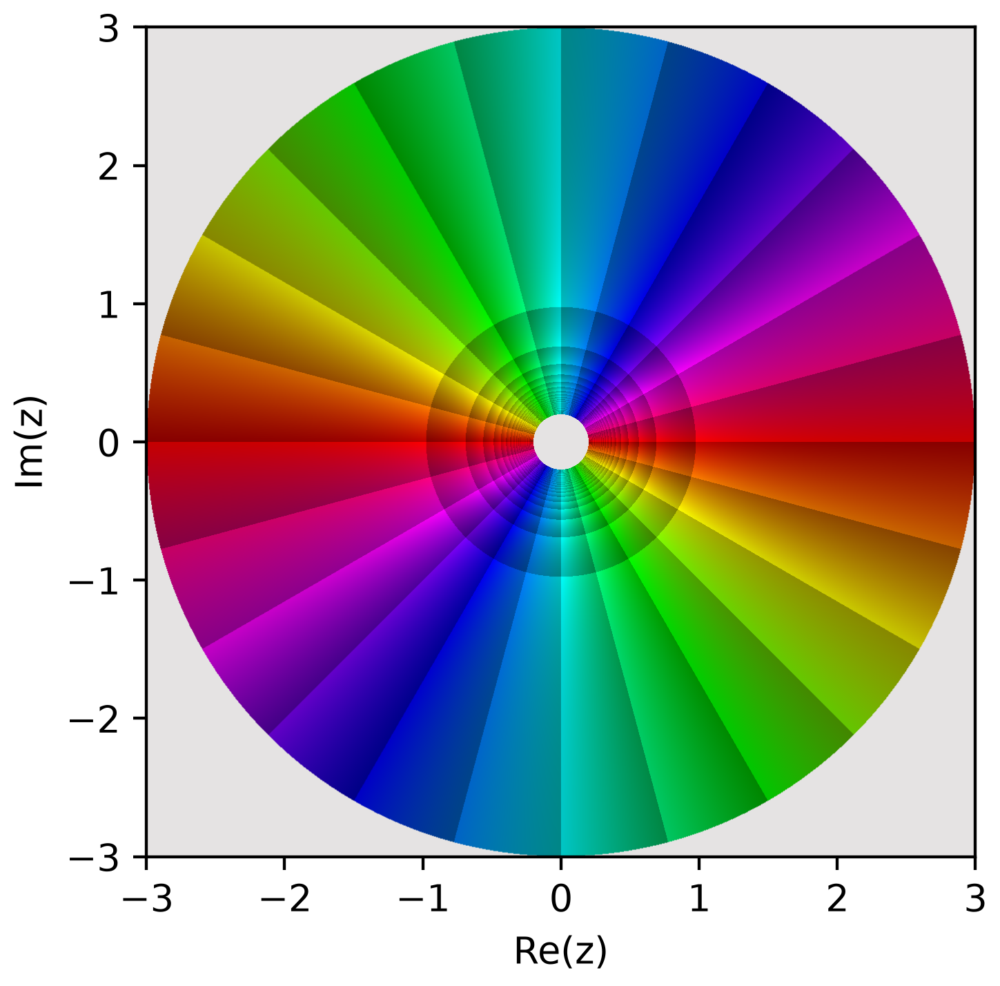
Double pole
An order-2 pole at the origin; phase winds backward twice.
Show the code
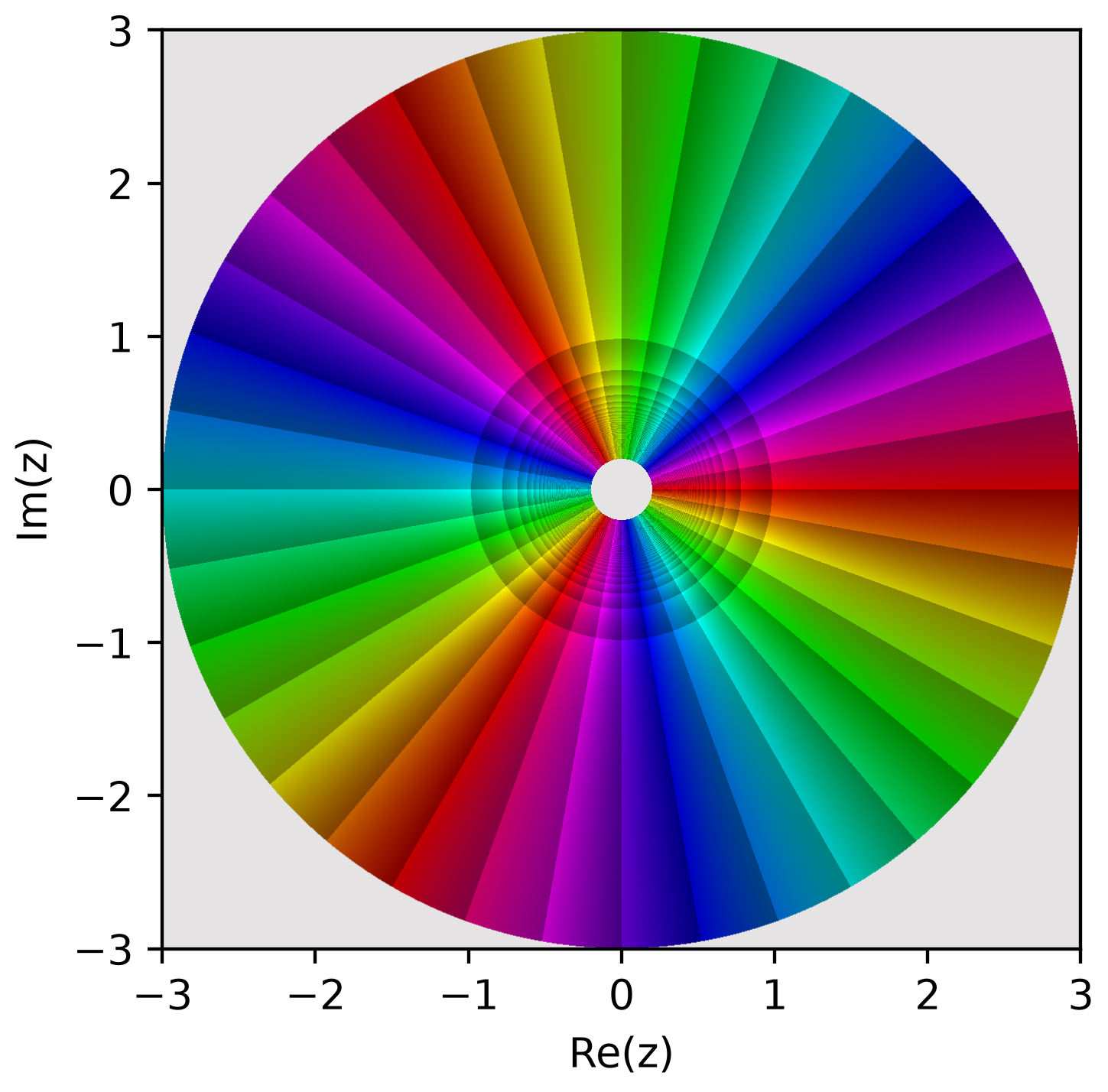
Triple pole
An order-3 pole at the origin.
Show the code
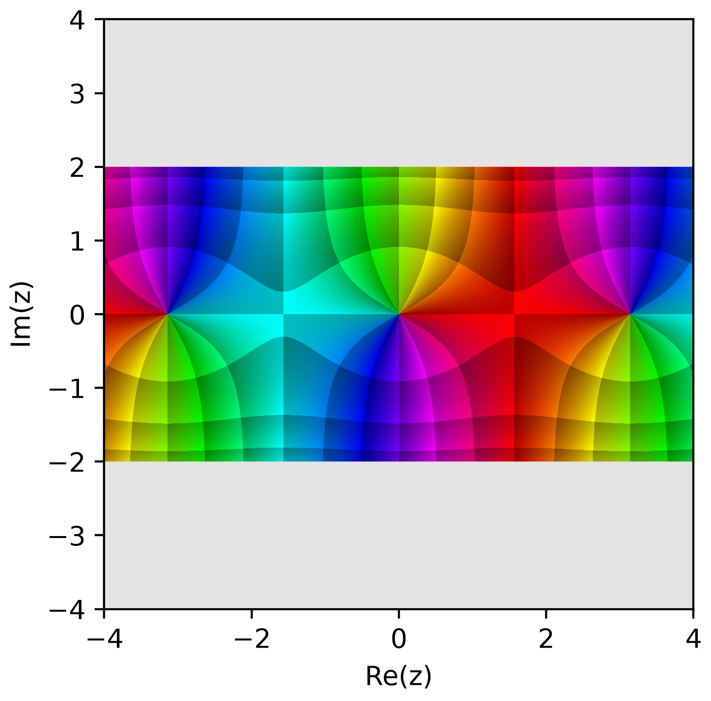
Sine
Simple zeros at integer multiples of pi (−pi, 0, pi shown).
Show the code
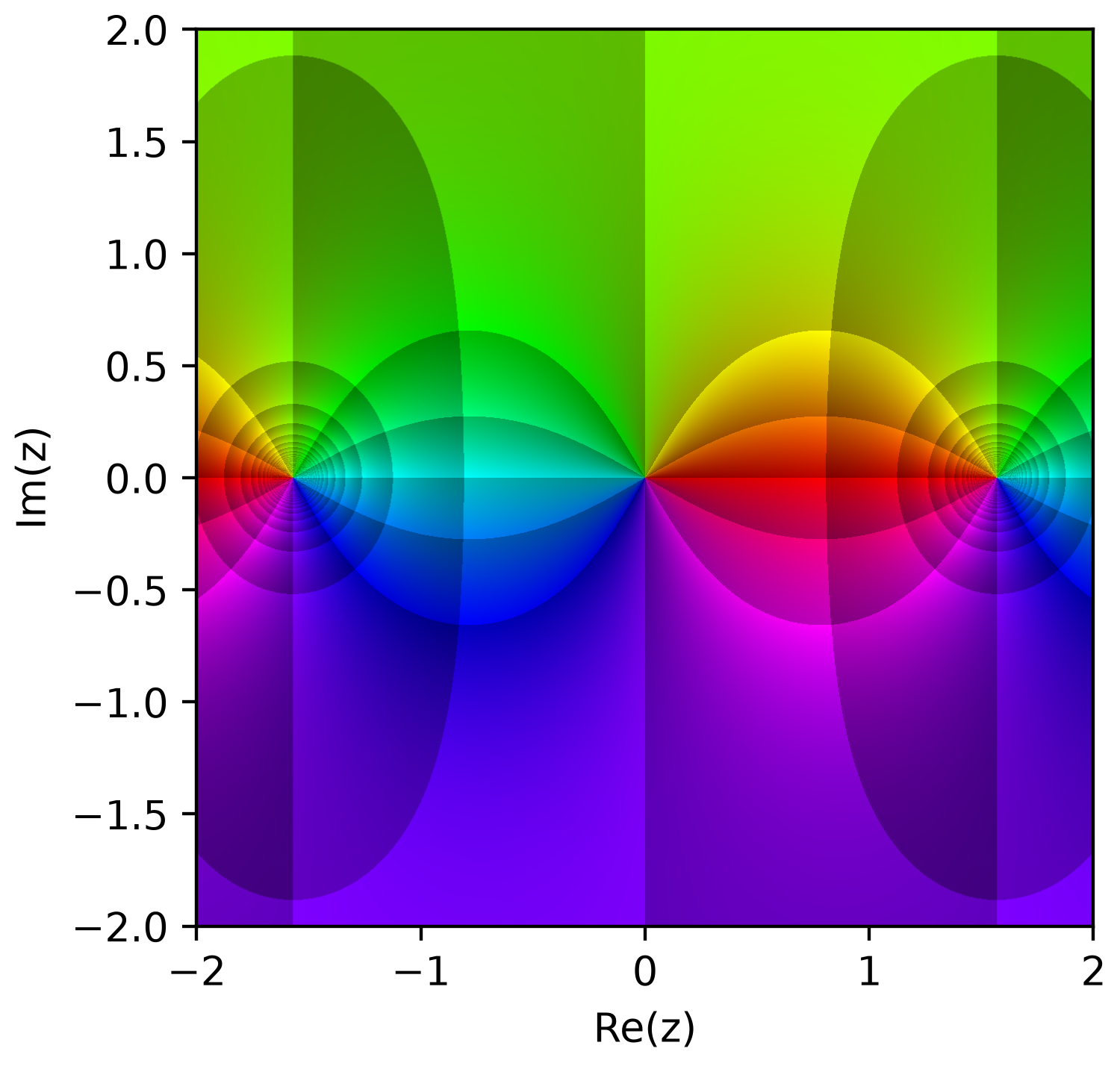
Tangent
Zero at 0; simple poles at ±pi/2 (within the shown window).
Show the code
Mapping and topology
The same functions lifted off the plane: magnitude as height, and the sphere that compactifies the plane so infinity has a place to sit.
From the plane to a landscape
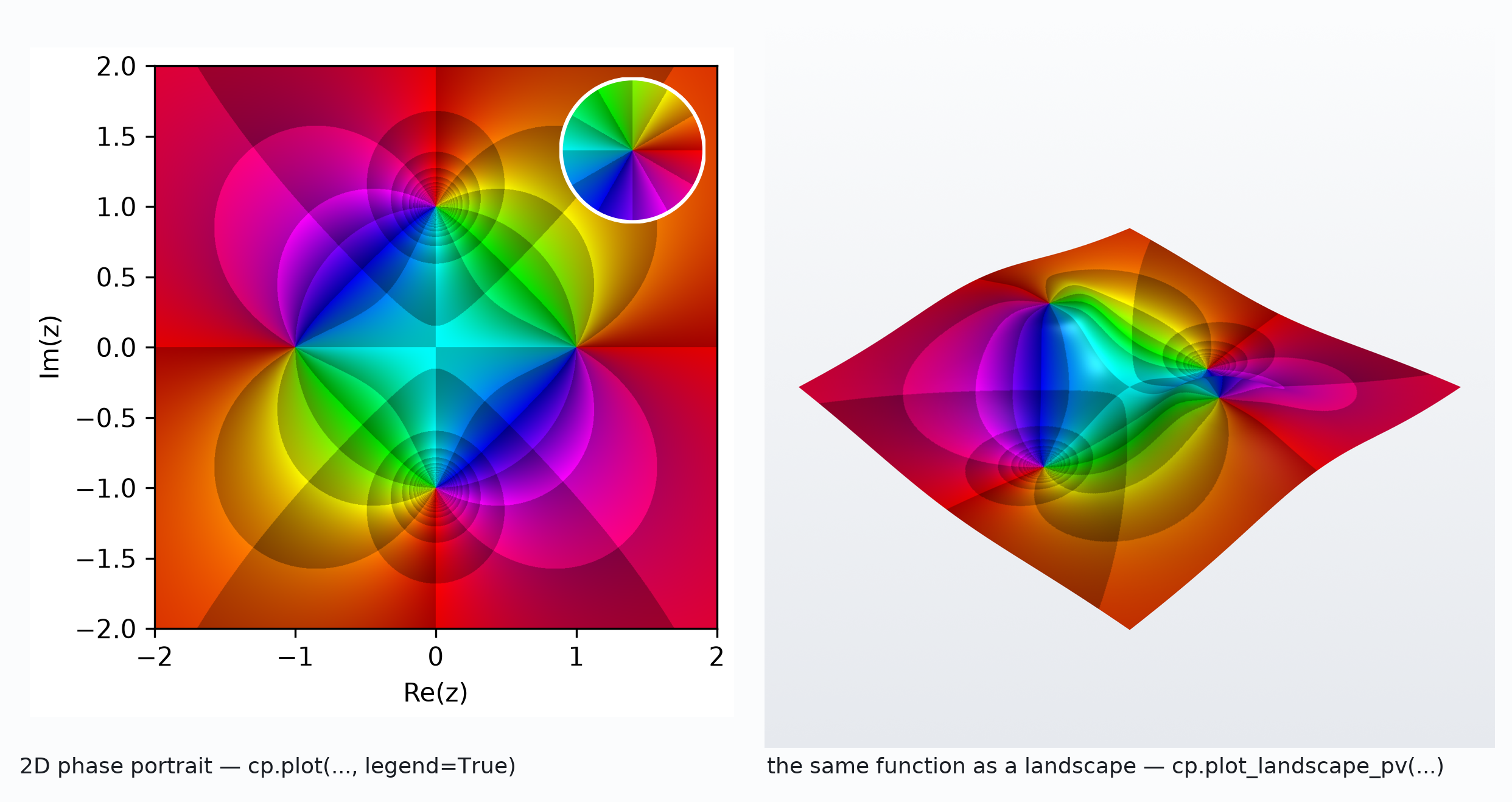
The same function twice: flat, then with |f(z)| lifted into height. The zeros sink and the poles rise, while the colours stay put — the landscape adds magnitude without changing what the hue means.
Show the code
import complexplorer as cp
preset = cp.catalog.get("rational_zeros_poles")
cp.plot(preset.domain(), preset.func, cmap=preset.colormap(), legend=True)
sc = preset.scaling()
cp.plot_landscape_pv(preset.domain(), preset.func, cmap=preset.colormap(),
modulus_mode=sc["method"], modulus_params=sc["params"])
Domains compose
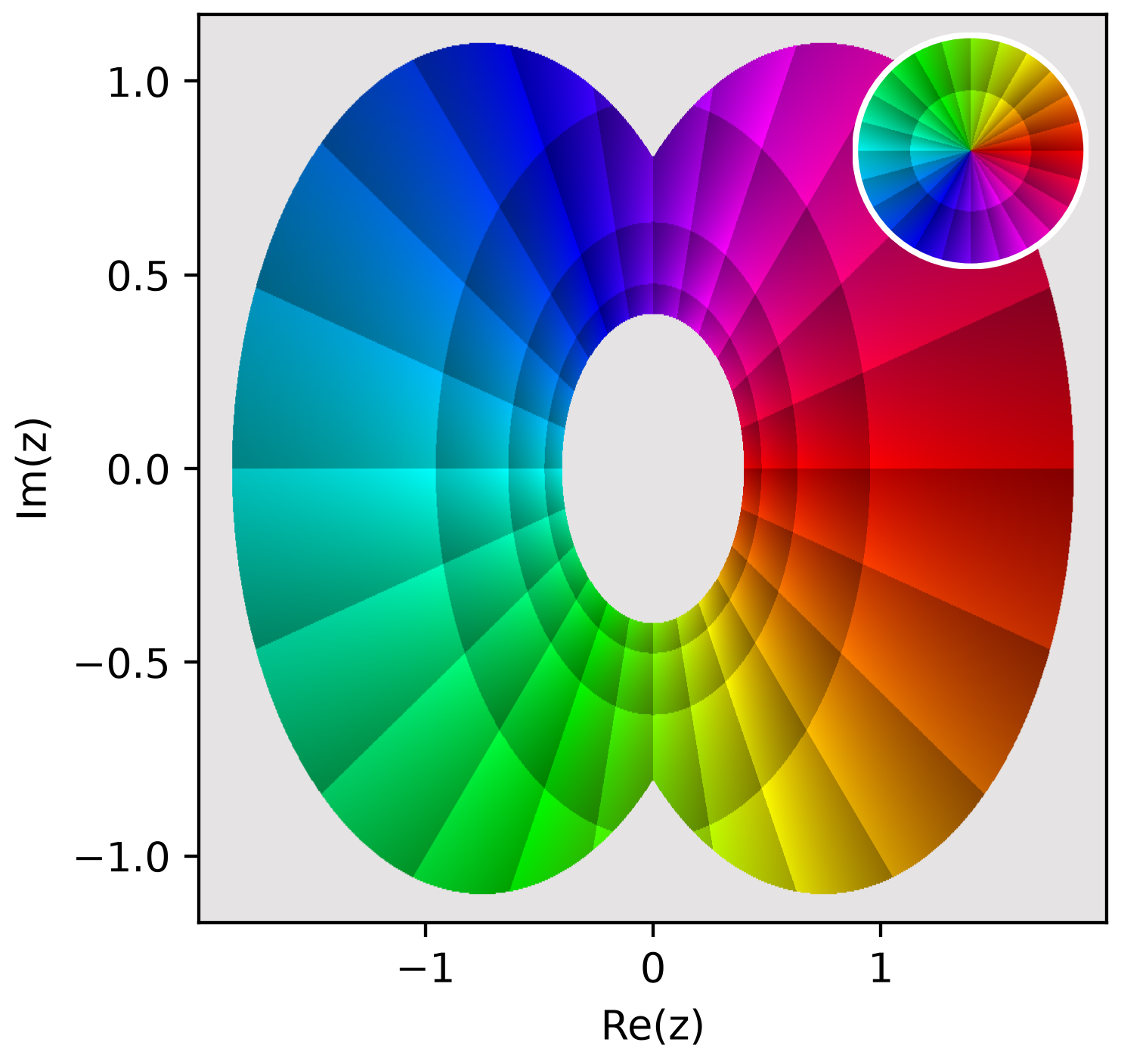
The outline is two overlapping disks unioned together, with a third punched out of the middle. Excluding a neighbourhood of the pole is not cosmetic: it keeps the huge values near z = 0 out of the sampling entirely.
Show the code
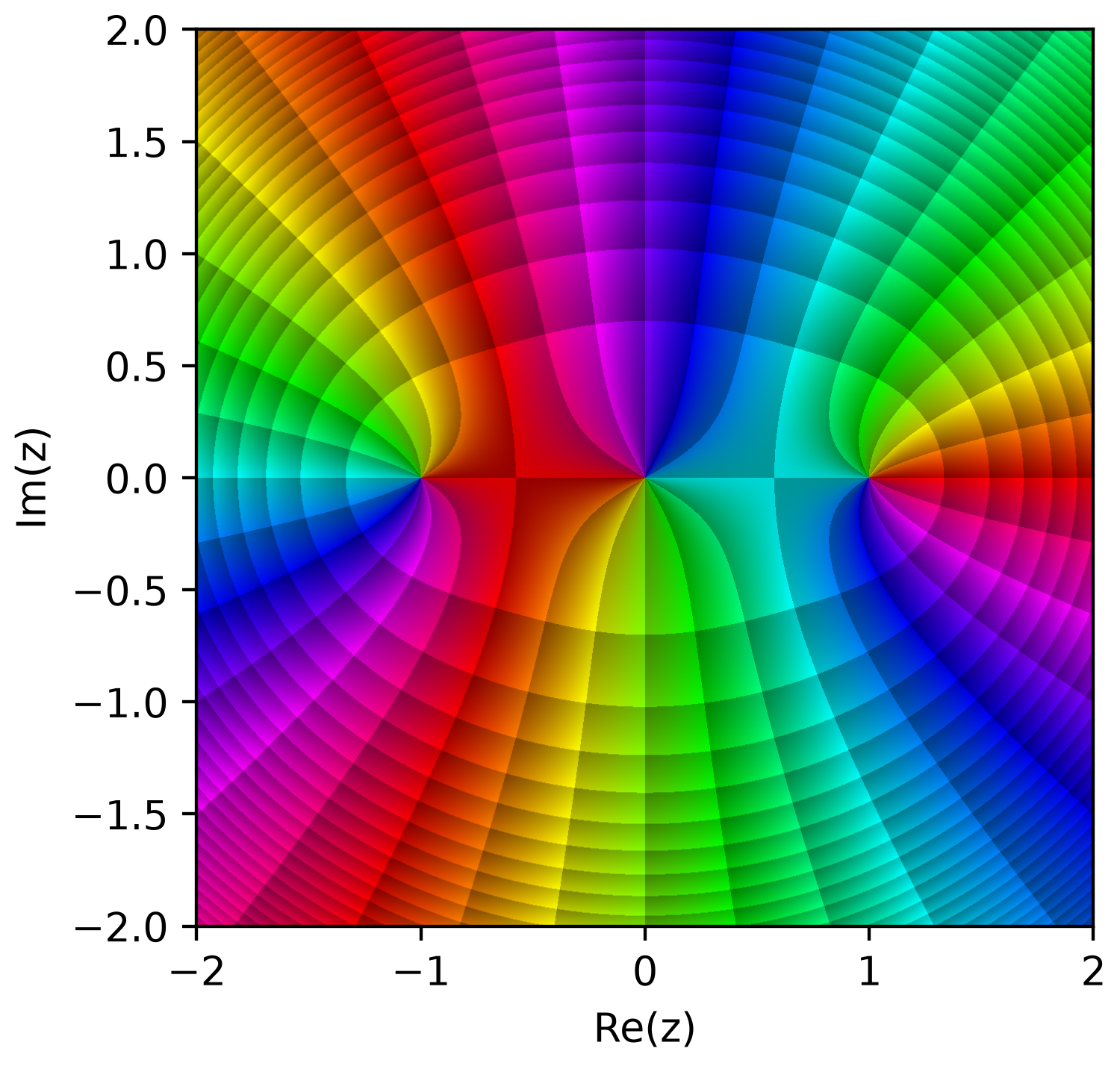
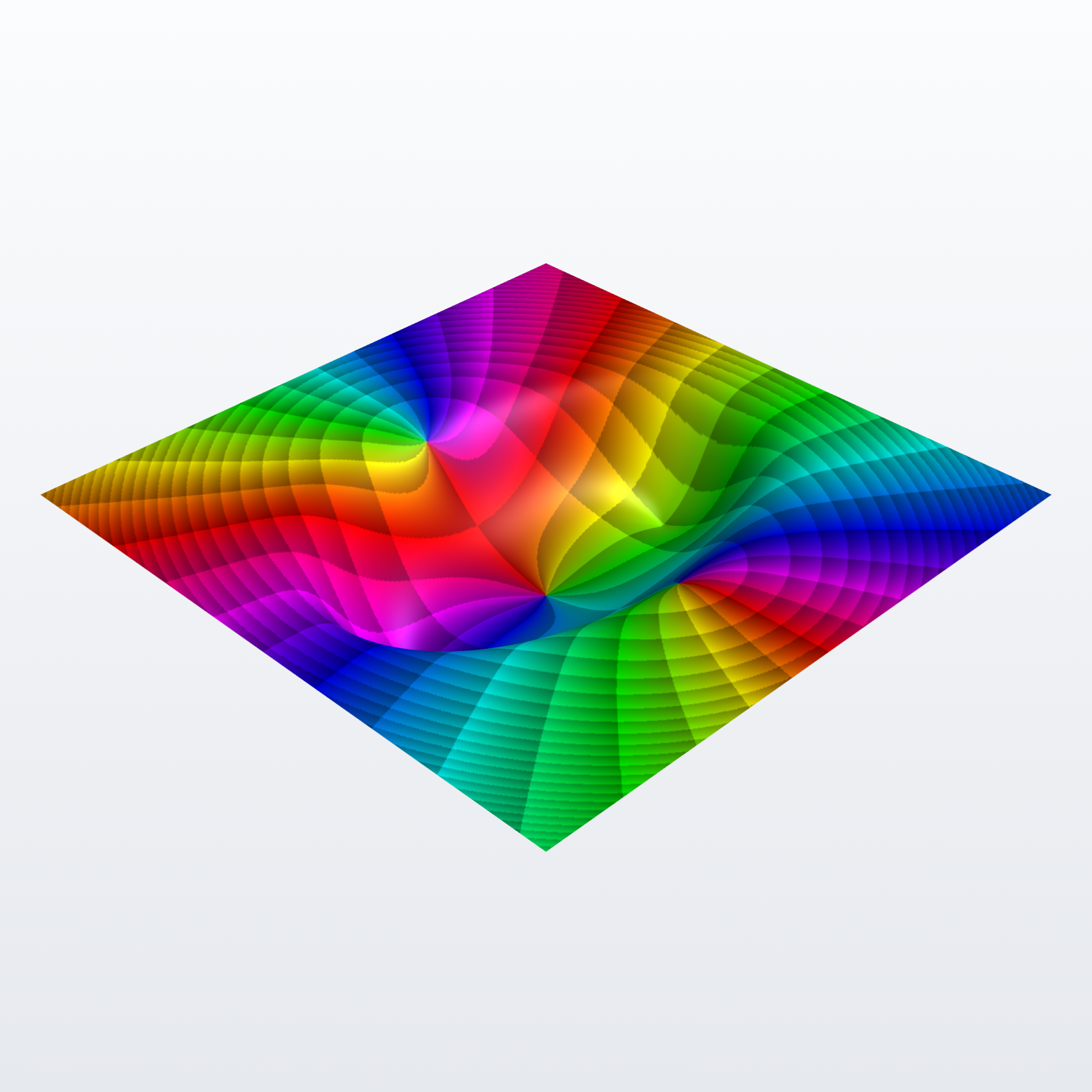
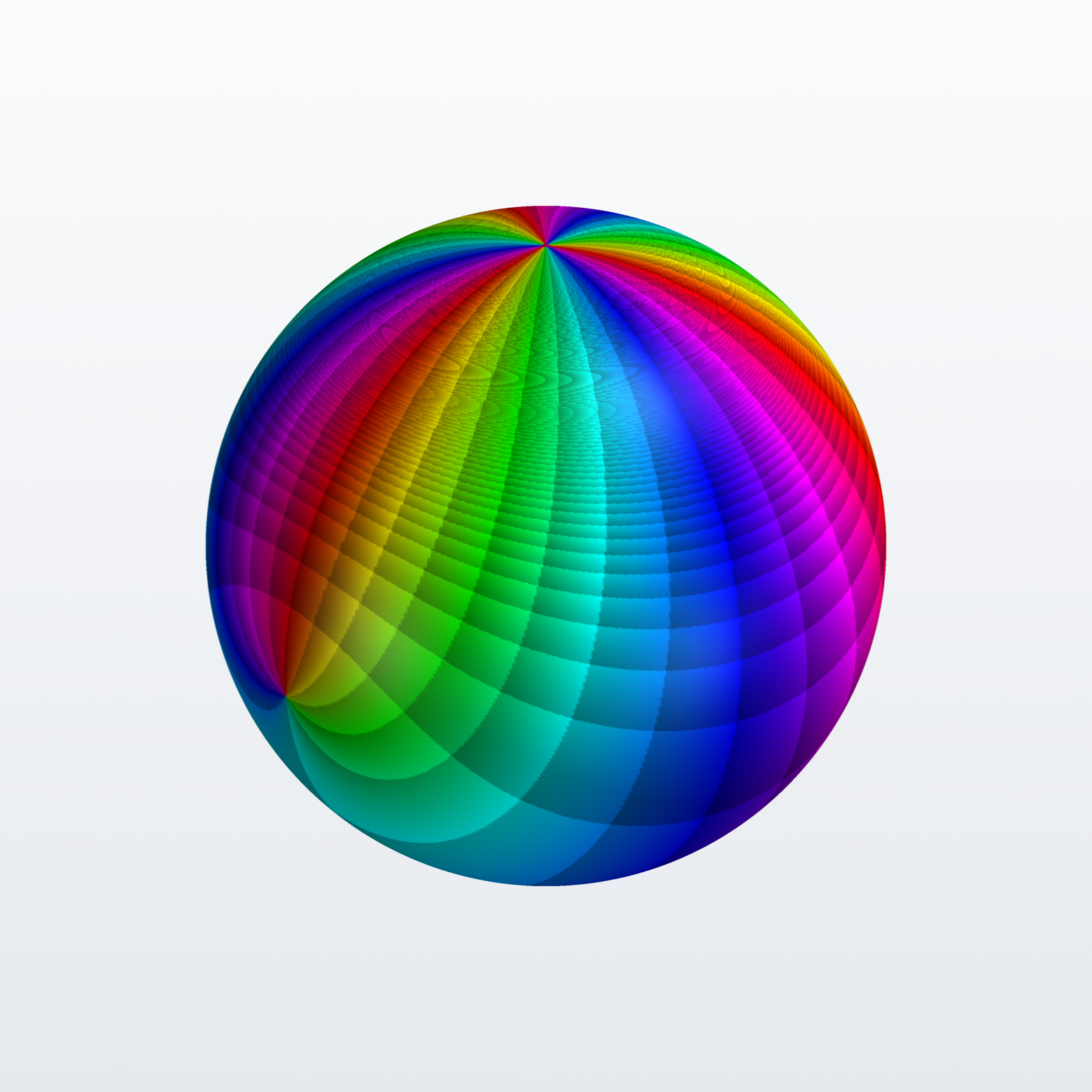
z³ - z
Three simple zeros at -1, 0, 1.
Show the code
import complexplorer as cp
preset = cp.catalog.get("cubic_real_roots")   # f(z) = z**3 - z
cp.plot(preset.domain(), preset.func, cmap=preset.colormap())

# ---
import complexplorer as cp
preset = cp.catalog.get("cubic_real_roots")   # f(z) = z**3 - z
sc = preset.scaling()
cp.plot_landscape_pv(preset.domain(), preset.func, cmap=preset.colormap(),
                     modulus_mode=sc["method"], modulus_params=sc["params"])

# ---
import complexplorer as cp
preset = cp.catalog.get("cubic_real_roots")   # f(z) = z**3 - z
cp.riemann_pv(preset.func, cmap=preset.colormap())   # full sphere
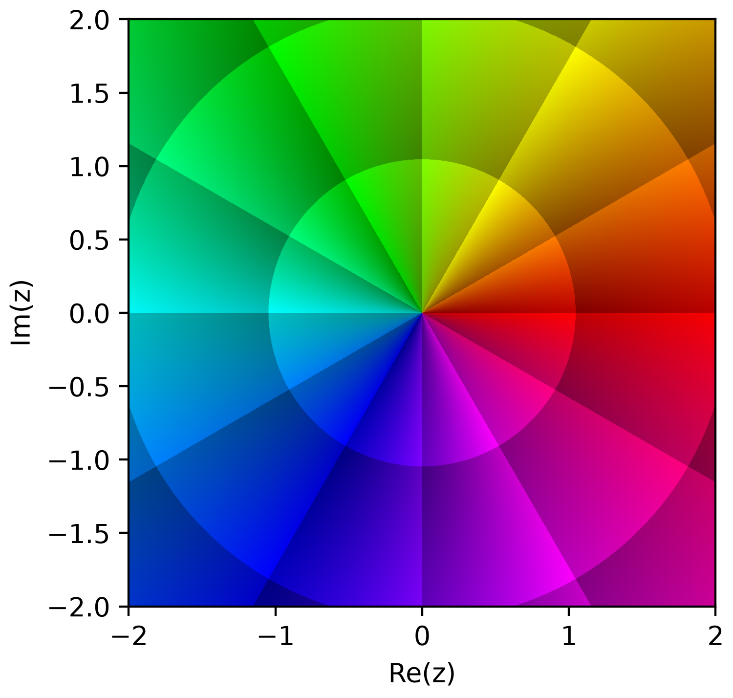
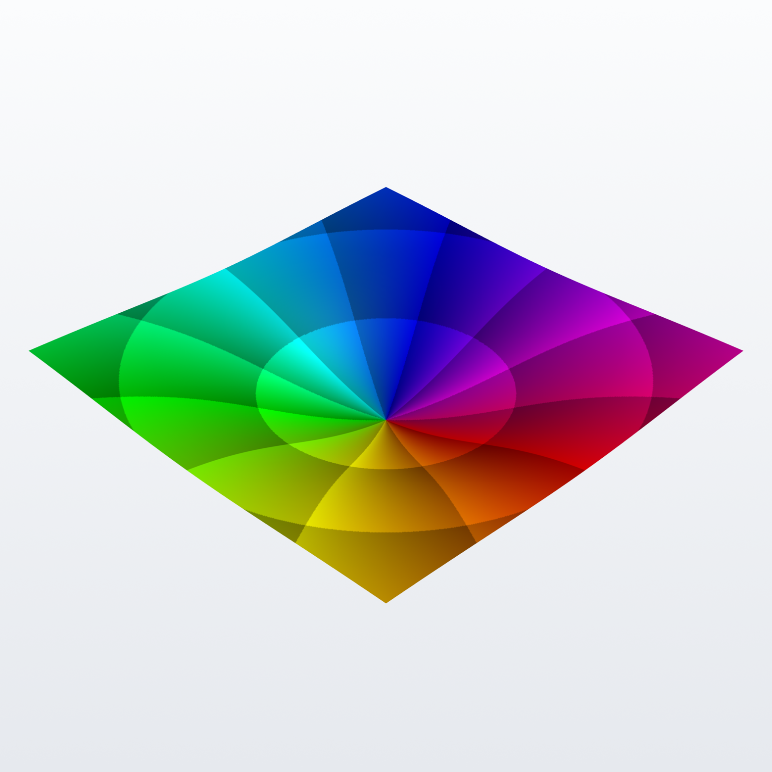
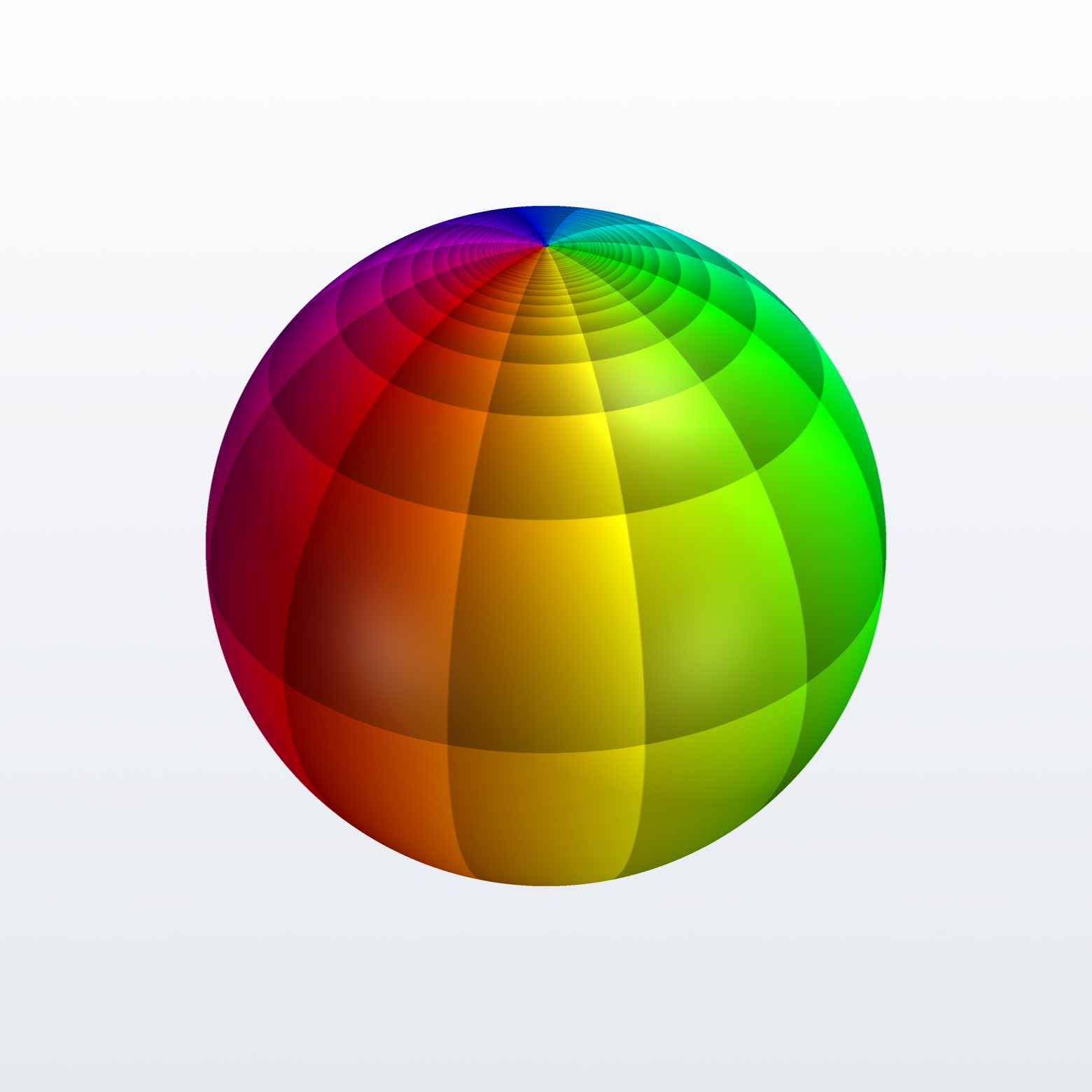
Identity
The identity map. A single simple zero at the origin; phase winds once.
Show the code
import complexplorer as cp
preset = cp.catalog.get("identity")   # f(z) = z
cp.plot(preset.domain(), preset.func, cmap=preset.colormap())

# ---
import complexplorer as cp
preset = cp.catalog.get("identity")   # f(z) = z
sc = preset.scaling()
cp.plot_landscape_pv(preset.domain(), preset.func, cmap=preset.colormap(),
                     modulus_mode=sc["method"], modulus_params=sc["params"])

# ---
import complexplorer as cp
preset = cp.catalog.get("identity")   # f(z) = z
cp.riemann_pv(preset.func, cmap=preset.colormap())   # full sphere
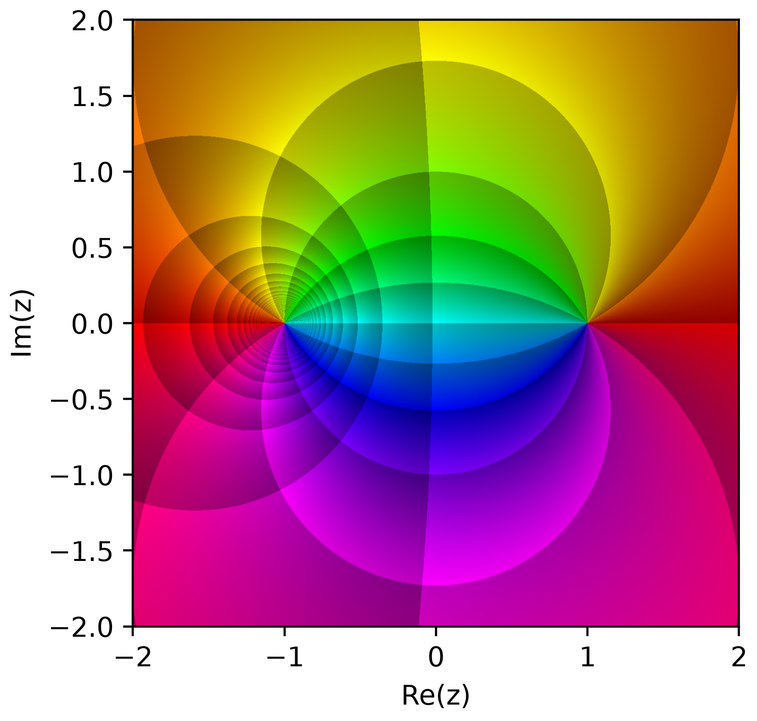
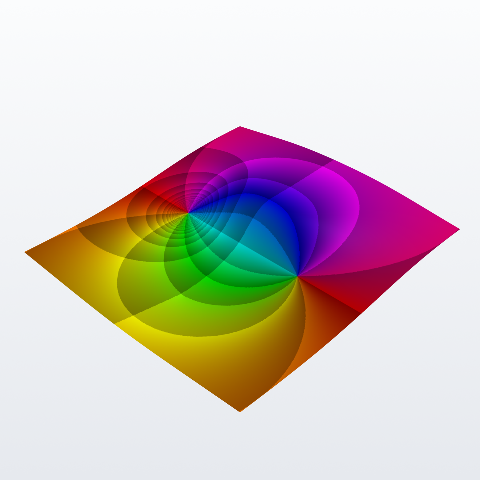
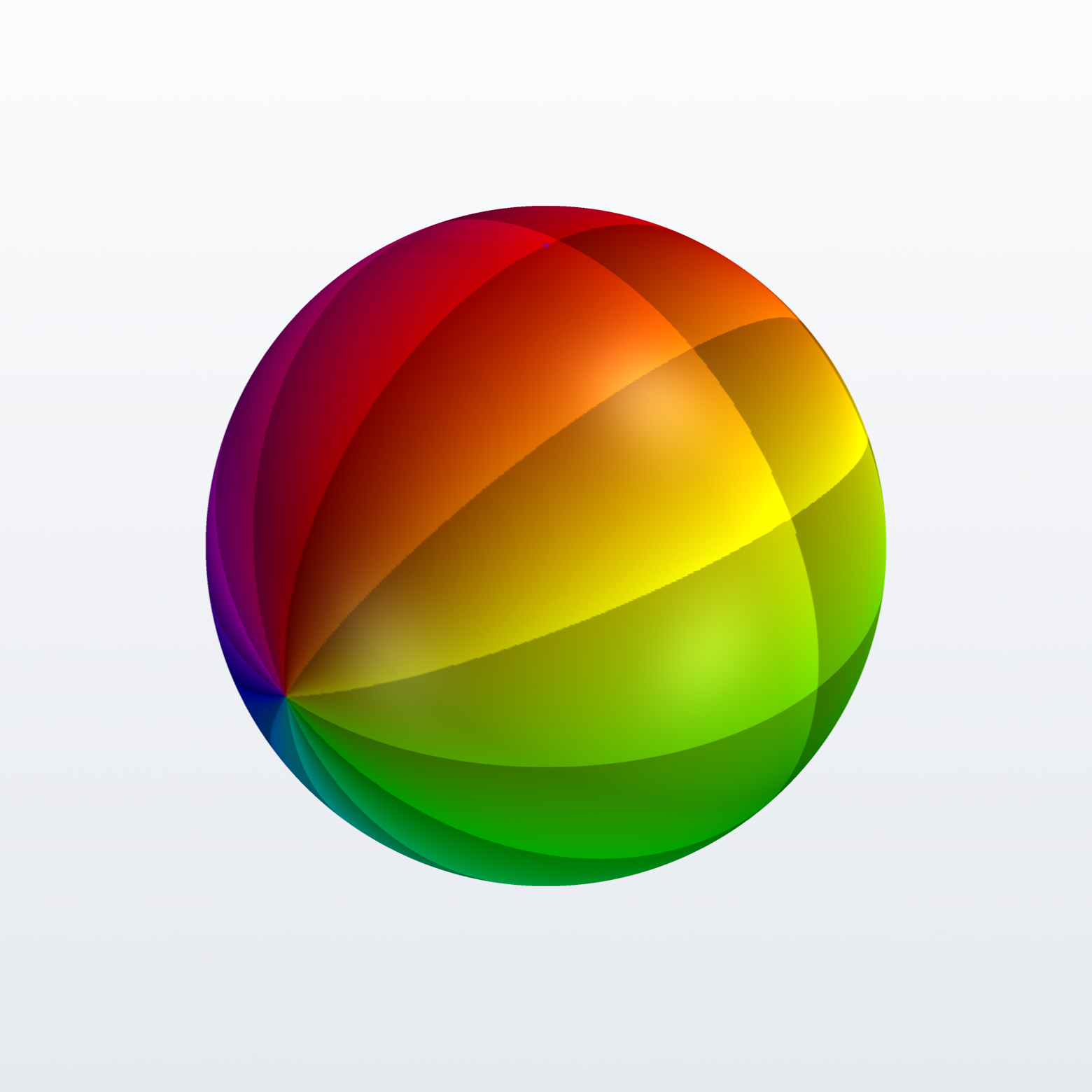
Cayley transform
One zero at +1, one pole at -1. Maps the right half-plane to the unit disk.
Show the code
import complexplorer as cp
preset = cp.catalog.get("mobius_cayley")   # f(z) = (z - 1) / (z + 1)
cp.plot(preset.domain(), preset.func, cmap=preset.colormap())

# ---
import complexplorer as cp
preset = cp.catalog.get("mobius_cayley")   # f(z) = (z - 1) / (z + 1)
sc = preset.scaling()
cp.plot_landscape_pv(preset.domain(), preset.func, cmap=preset.colormap(),
                     modulus_mode=sc["method"], modulus_params=sc["params"])

# ---
import complexplorer as cp
preset = cp.catalog.get("mobius_cayley")   # f(z) = (z - 1) / (z + 1)
cp.riemann_pv(preset.func, cmap=preset.colormap())   # full sphere
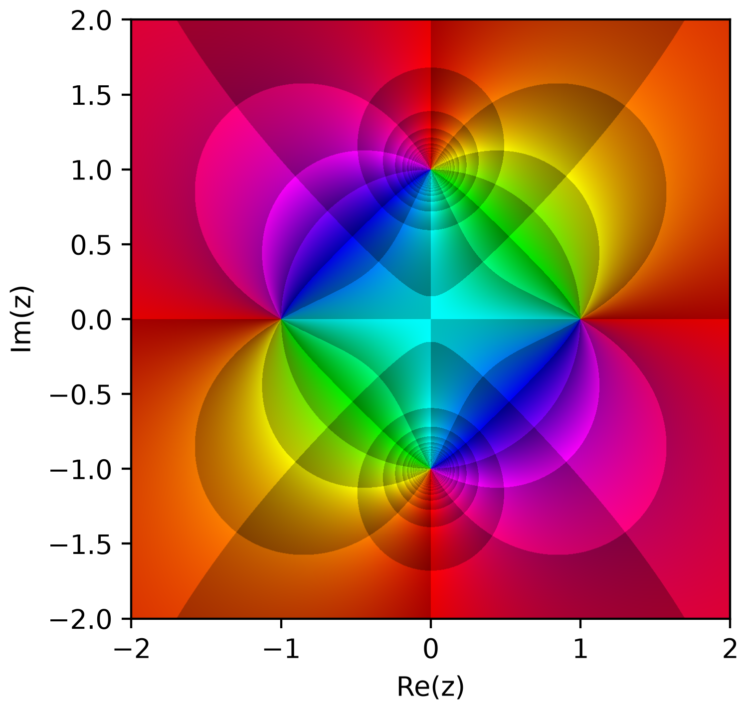
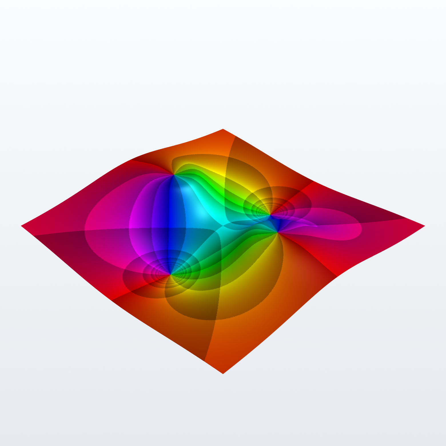
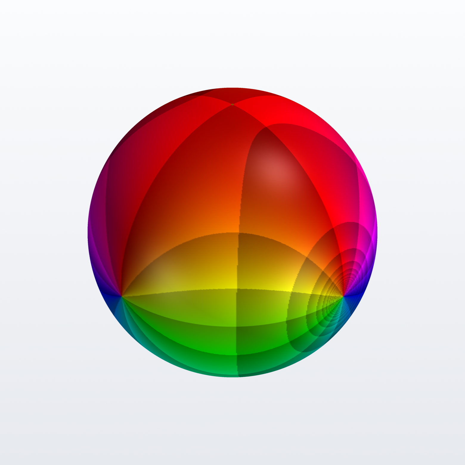
(z² - 1)/(z² + 1)
Zeros at ±1, poles at ±i.
Show the code
import complexplorer as cp
preset = cp.catalog.get("rational_zeros_poles")   # f(z) = (z**2 - 1) / (z**2 + 1)
cp.plot(preset.domain(), preset.func, cmap=preset.colormap())

# ---
import complexplorer as cp
preset = cp.catalog.get("rational_zeros_poles")   # f(z) = (z**2 - 1) / (z**2 + 1)
sc = preset.scaling()
cp.plot_landscape_pv(preset.domain(), preset.func, cmap=preset.colormap(),
                     modulus_mode=sc["method"], modulus_params=sc["params"])

# ---
import complexplorer as cp
preset = cp.catalog.get("rational_zeros_poles")   # f(z) = (z**2 - 1) / (z**2 + 1)
cp.riemann_pv(preset.func, cmap=preset.colormap())   # full sphere
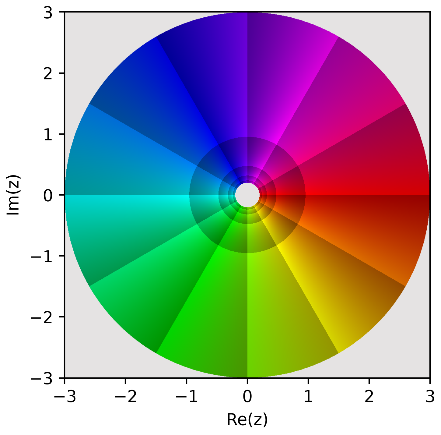
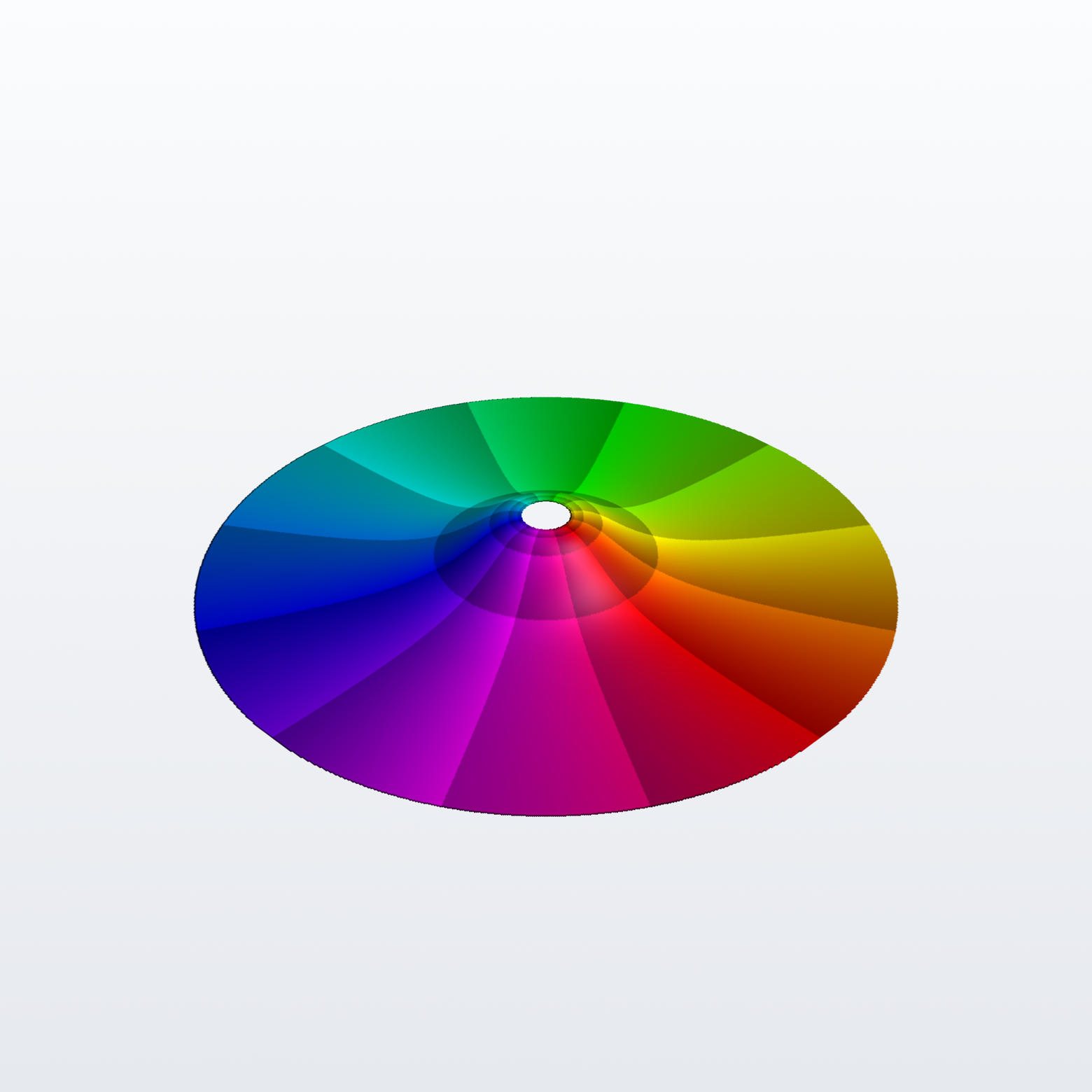
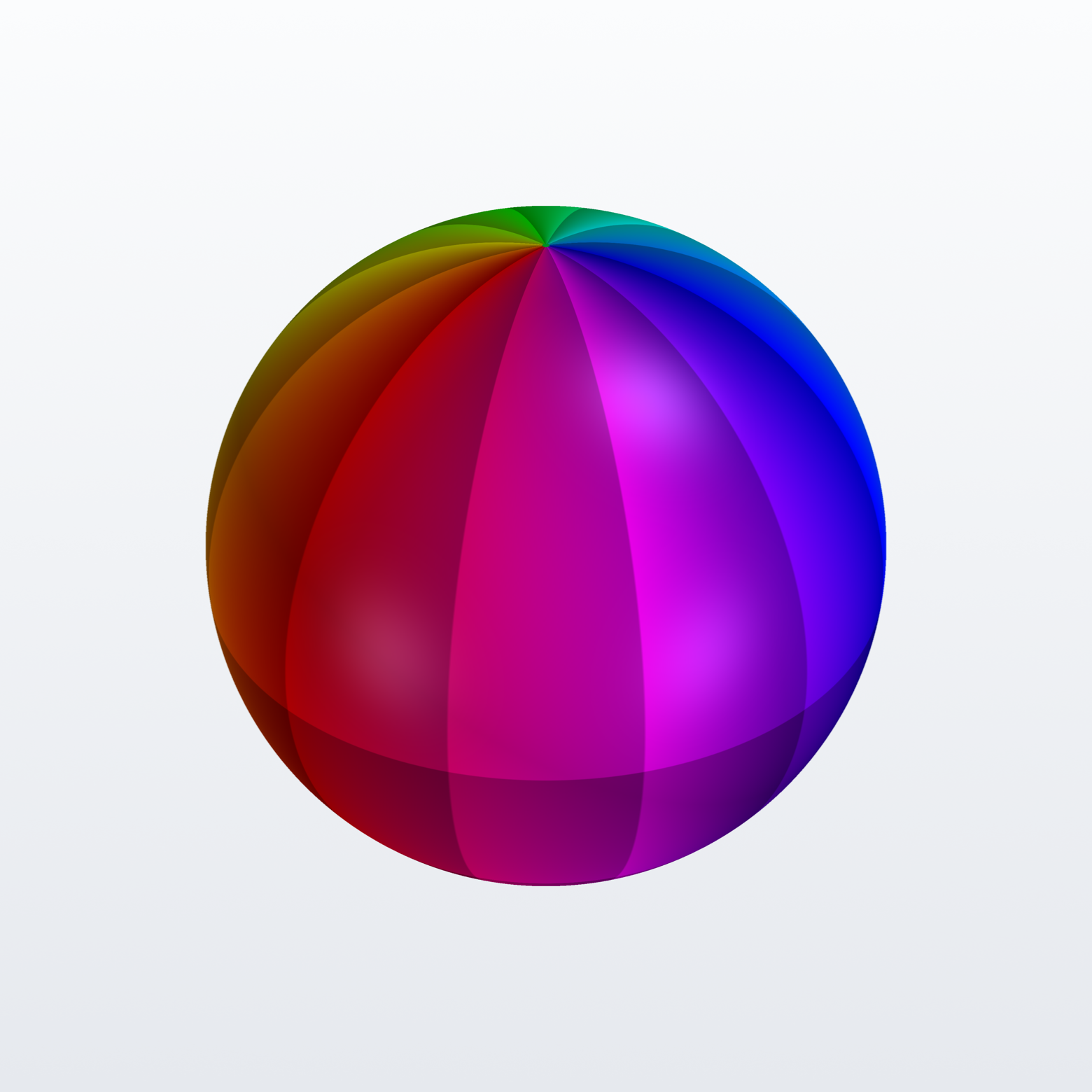
1 / z
A simple pole at the origin (Möbius inversion); phase winds backward.
Show the code
import complexplorer as cp
preset = cp.catalog.get("reciprocal")   # f(z) = 1 / z
cp.plot(preset.domain(), preset.func, cmap=preset.colormap())

# ---
import complexplorer as cp
preset = cp.catalog.get("reciprocal")   # f(z) = 1 / z
sc = preset.scaling()
cp.plot_landscape_pv(preset.domain(), preset.func, cmap=preset.colormap(),
                     modulus_mode=sc["method"], modulus_params=sc["params"])

# ---
import complexplorer as cp
preset = cp.catalog.get("reciprocal")   # f(z) = 1 / z
cp.riemann_pv(preset.func, cmap=preset.colormap())   # full sphere
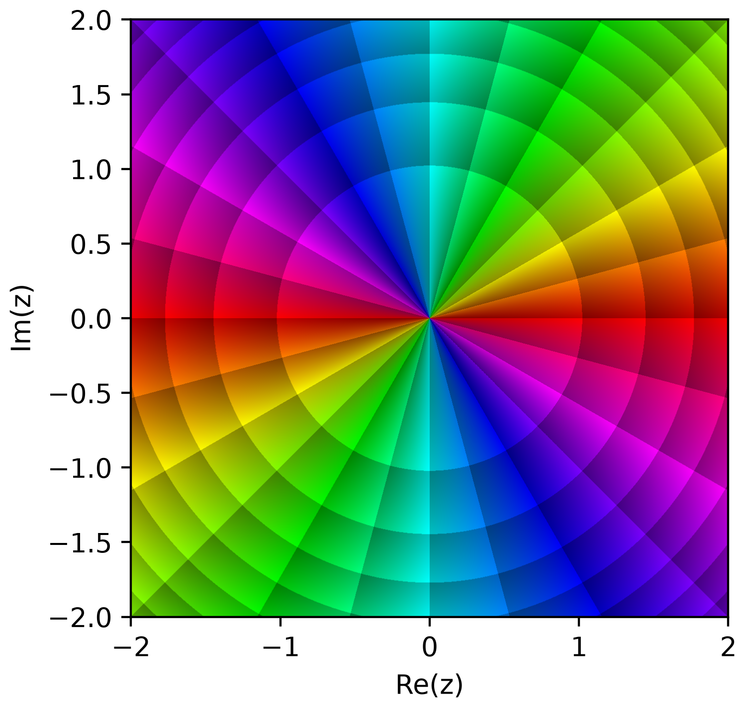
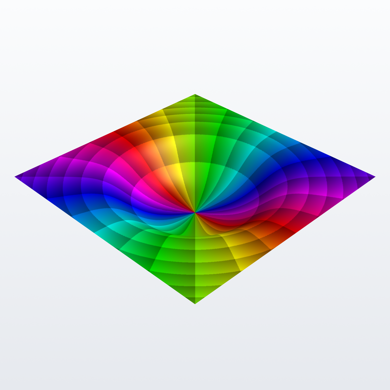
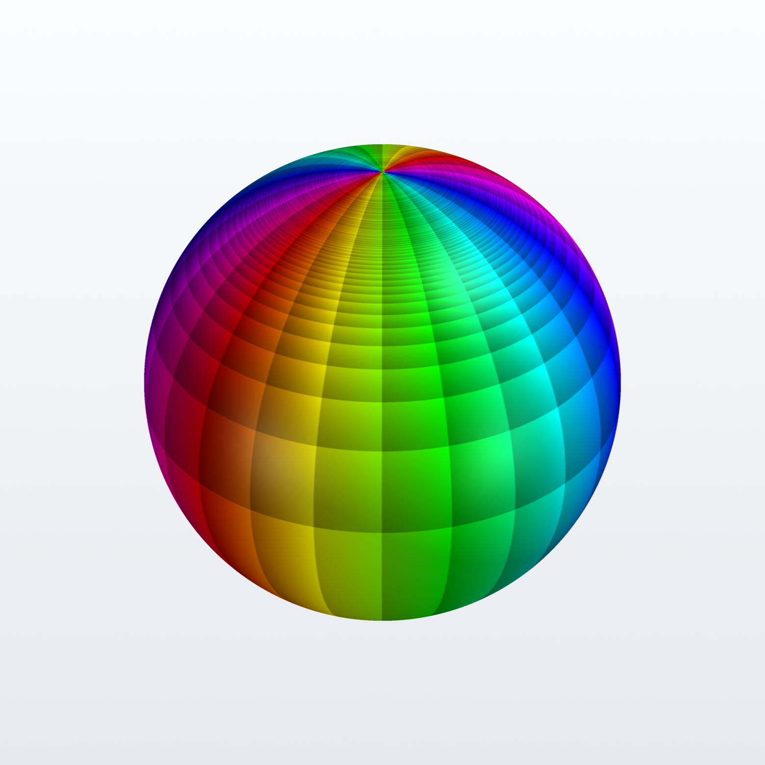
z squared
A double zero at the origin; phase winds twice.
Show the code
import complexplorer as cp
preset = cp.catalog.get("square")   # f(z) = z**2
cp.plot(preset.domain(), preset.func, cmap=preset.colormap())

# ---
import complexplorer as cp
preset = cp.catalog.get("square")   # f(z) = z**2
sc = preset.scaling()
cp.plot_landscape_pv(preset.domain(), preset.func, cmap=preset.colormap(),
                     modulus_mode=sc["method"], modulus_params=sc["params"])

# ---
import complexplorer as cp
preset = cp.catalog.get("square")   # f(z) = z**2
cp.riemann_pv(preset.func, cmap=preset.colormap())   # full sphere
Riemann surfaces
Multivalued families become single-valued on their covering surface. Branch points and cuts are geometry here, not bookkeeping.
Sphere versus surface
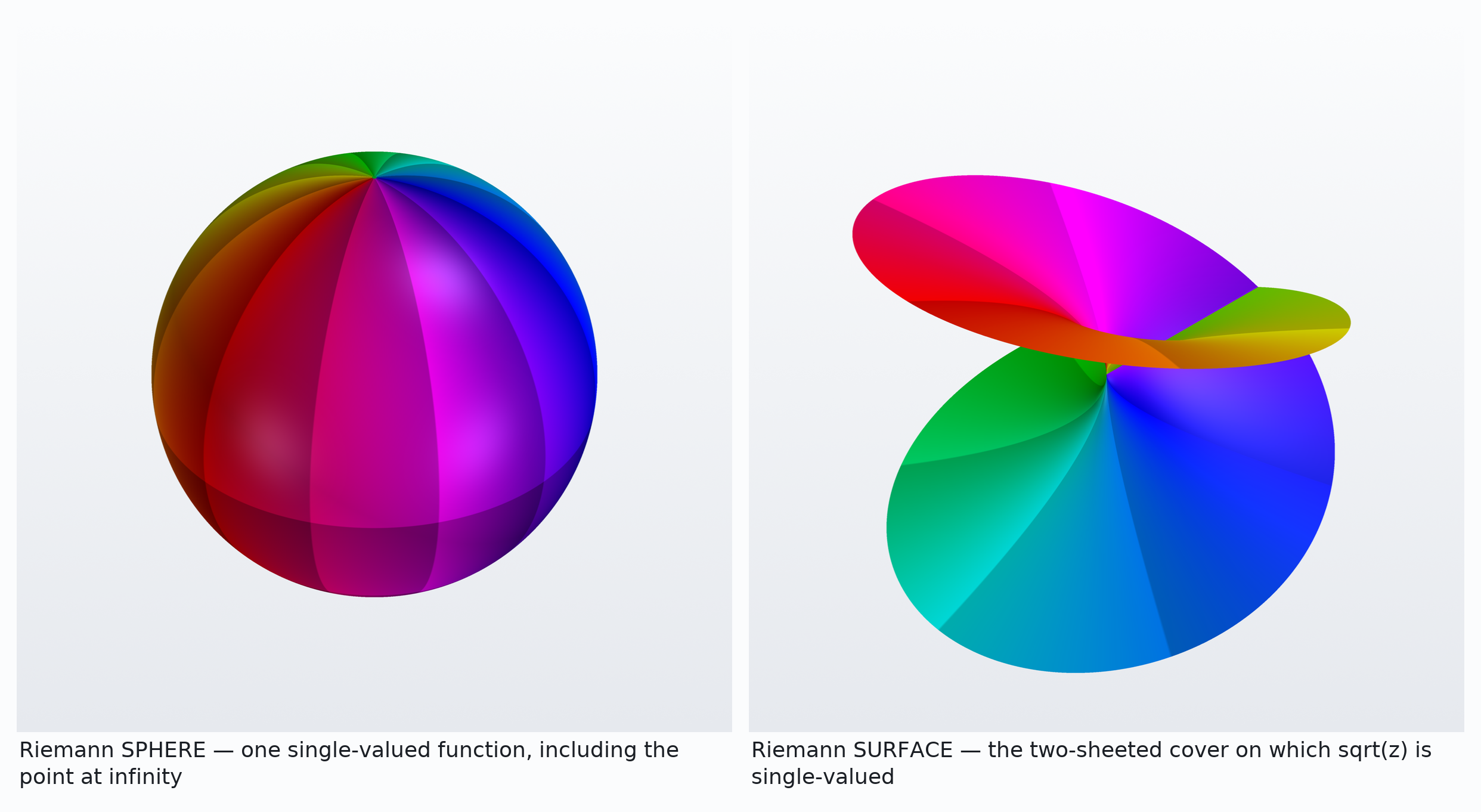
Two different objects that are easy to confuse. The sphere compactifies the plane so one single-valued function can include the point at infinity. The surface is the two-sheeted cover on which the multivalued sqrt(z) becomes single-valued.
Show the code
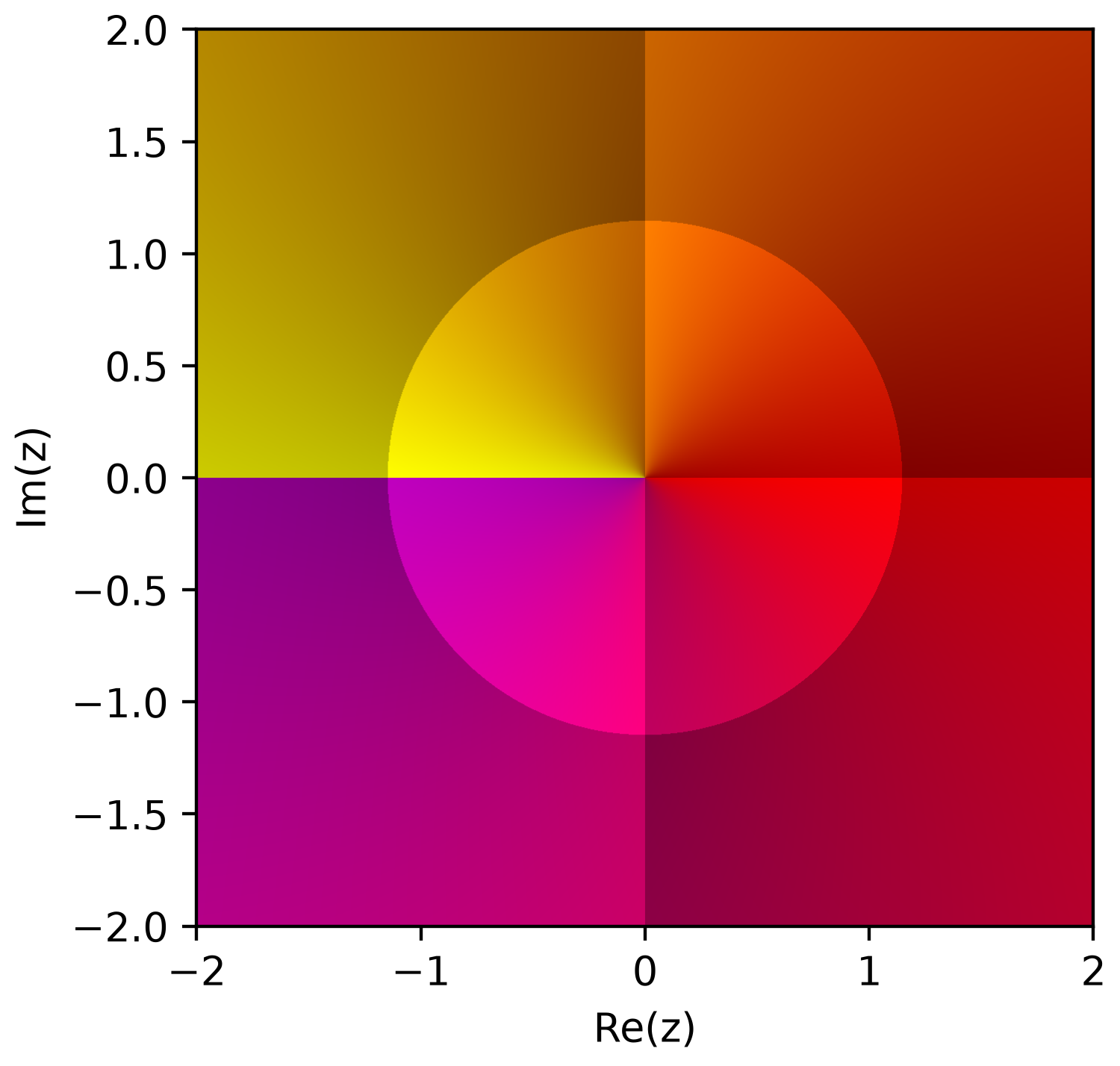
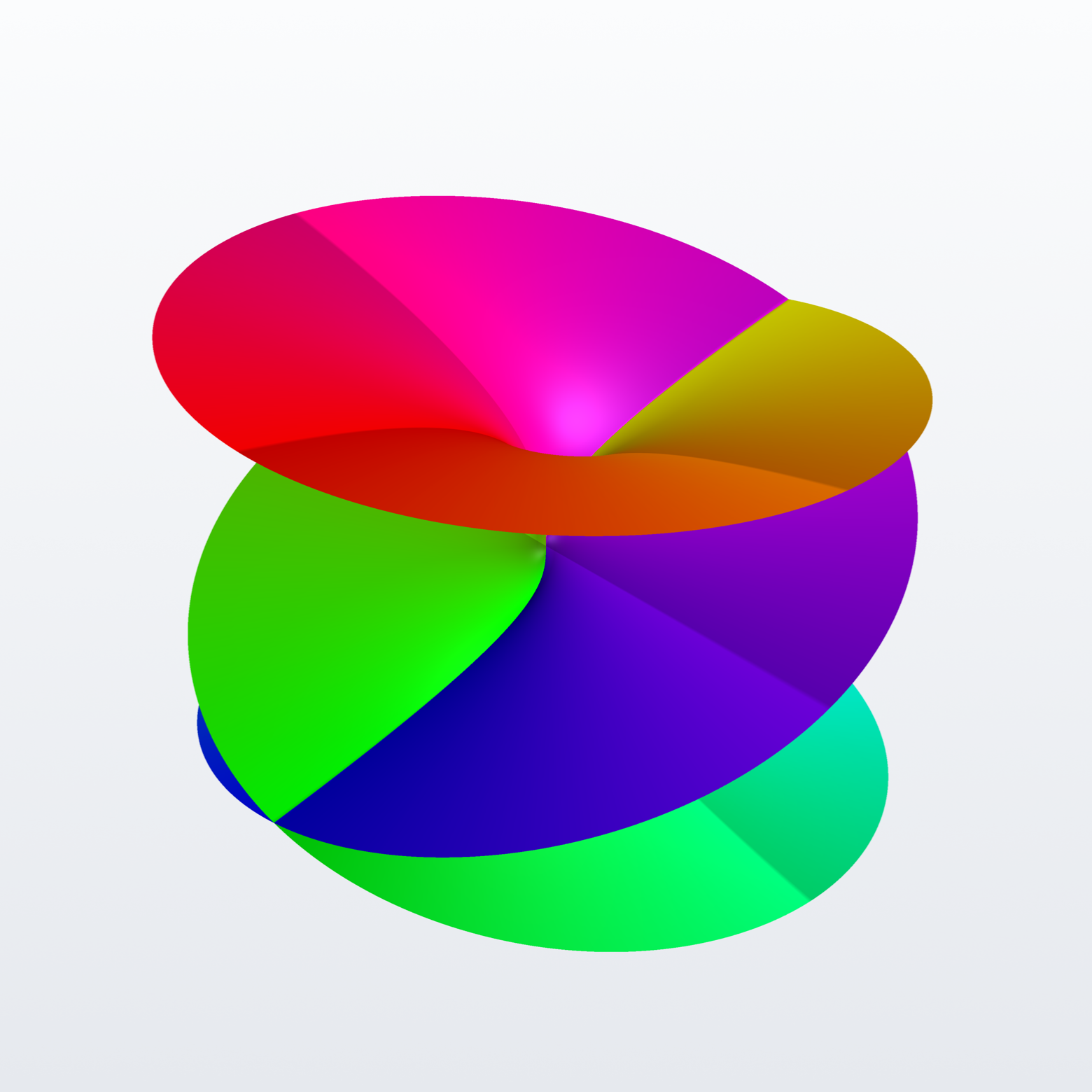
Cube root
Principal-branch cube root; an order-3 branch point at 0 (three sheets).
Show the code
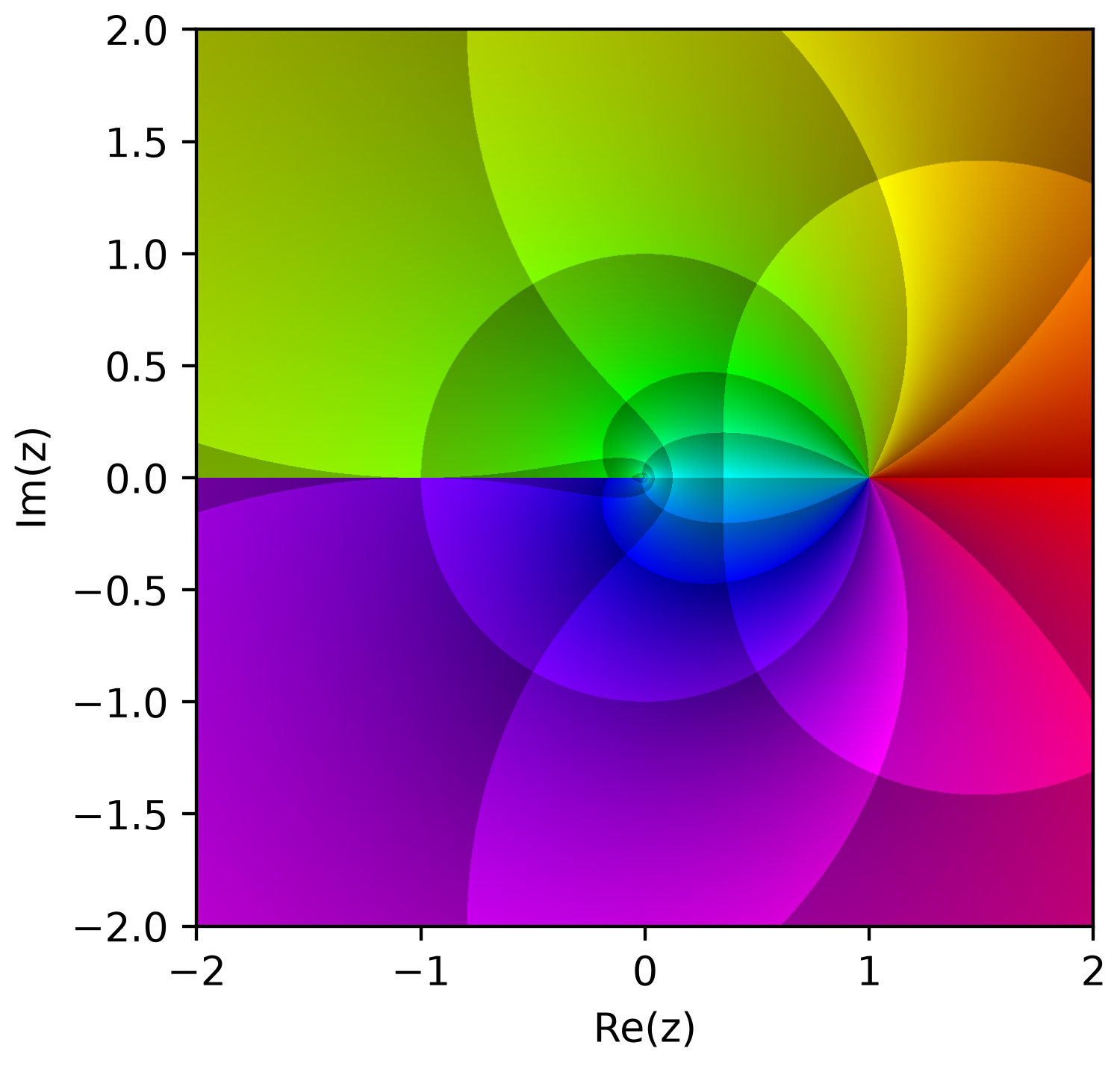
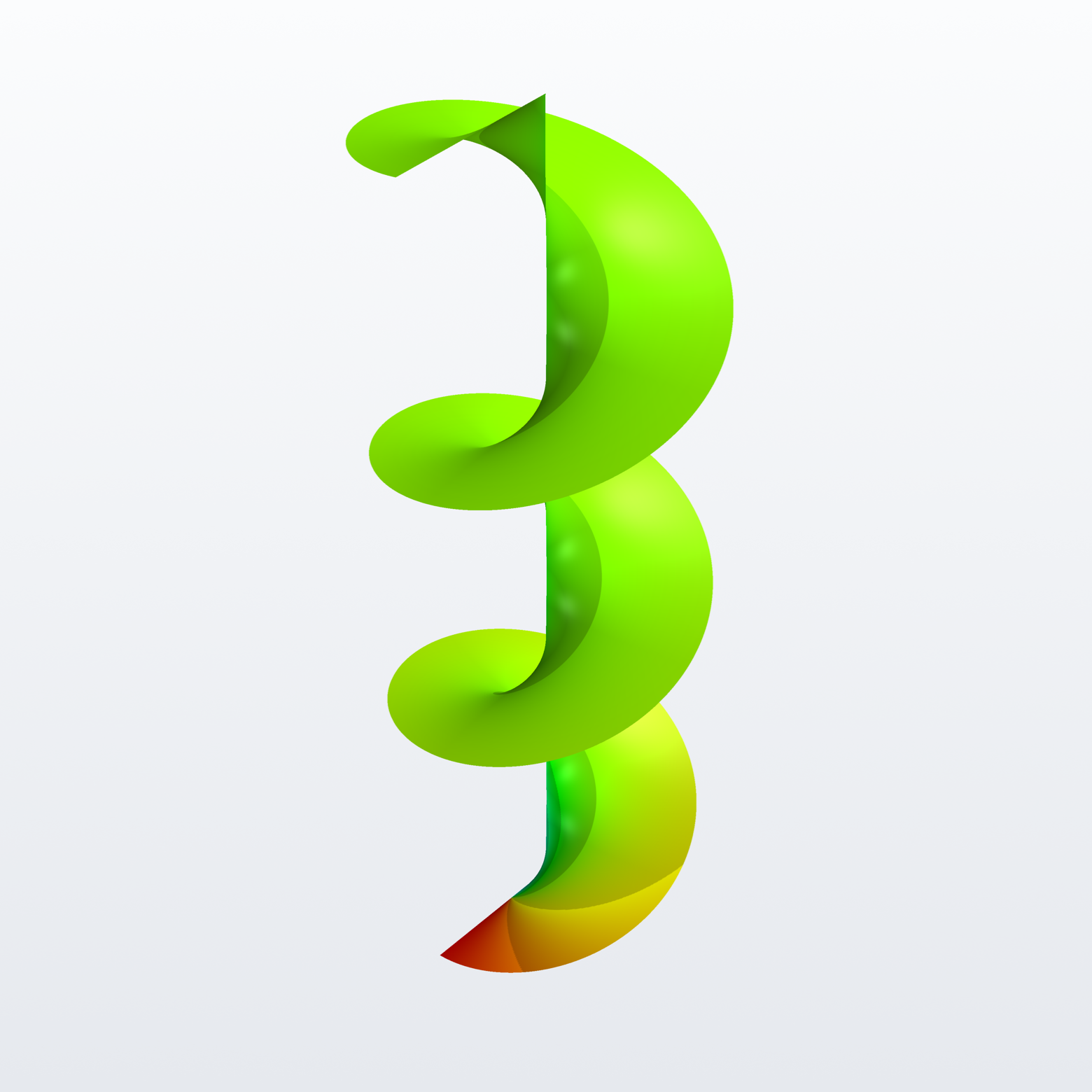
Natural log
Principal-branch logarithm; a logarithmic (infinite-order) branch point at 0.
Show the code
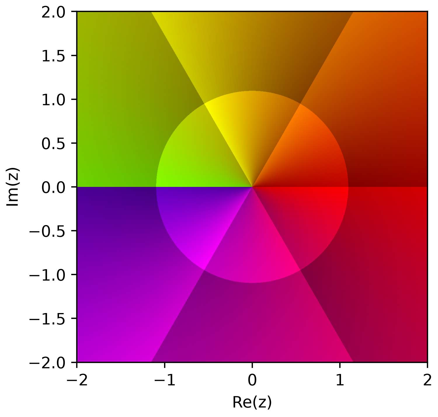
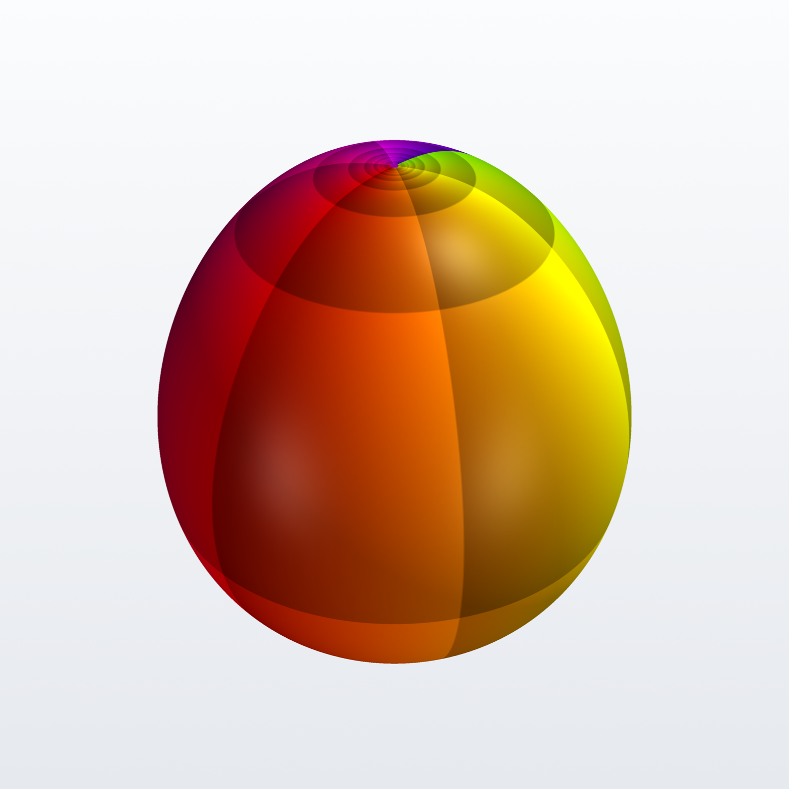
Square root
Principal-branch square root; an order-2 branch point at 0 (two sheets).

Show the code
import complexplorer as cp
preset = cp.catalog.get("sqrt")   # f(z) = sqrt(z)
cp.plot(preset.domain(), preset.func, cmap=preset.colormap())

# ---
import complexplorer as cp
cp.riemann_surface_pv("power", n=2)   # sqrt(z)

# ---
import complexplorer as cp
preset = cp.catalog.get("sqrt")   # f(z) = sqrt(z)
sc = preset.scaling()
cp.riemann_pv(preset.func, cmap=preset.colormap(),
              modulus_mode=sc["method"], modulus_params=sc["params"])  # relief
Engineering mode
A transfer function is a complex function, so the whole library applies to it.
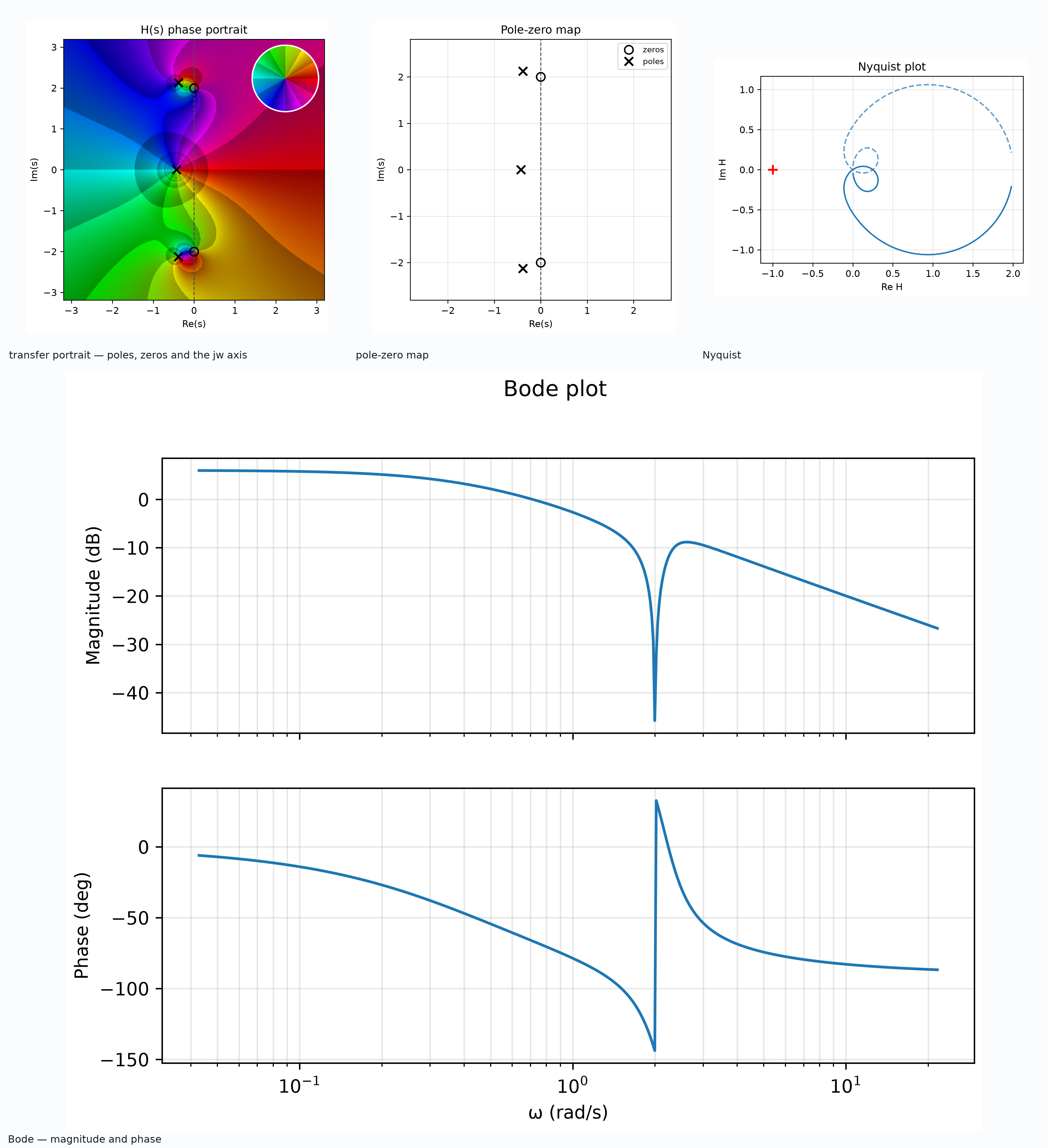
Engineering mode: a notch filter
One stable transfer function in four views. The zeros sit exactly on the jw axis at +-2j — the notch — while the poles stay inside the left half-plane. The portrait shows where they are; Bode and Nyquist show what they do to a signal.
Show the code
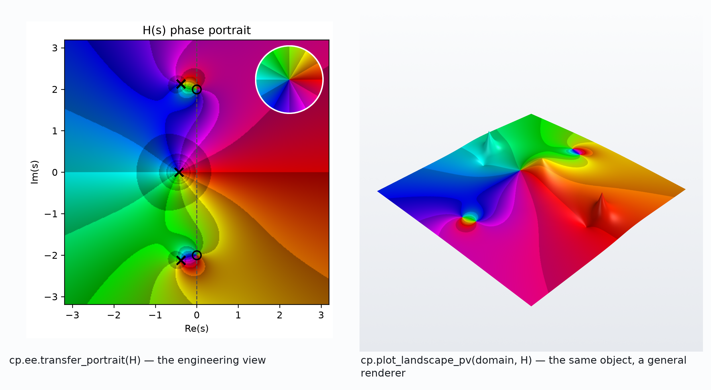
A transfer function is just a complex function
TransferFunction is a plain callable, so the engineering view and the general 3D renderer are looking at the same object. Nothing converts between them: the notch that reads as a dark point on the left is the valley on the right.
Show the code
Colormaps
One reference function under every colormap the package exports.
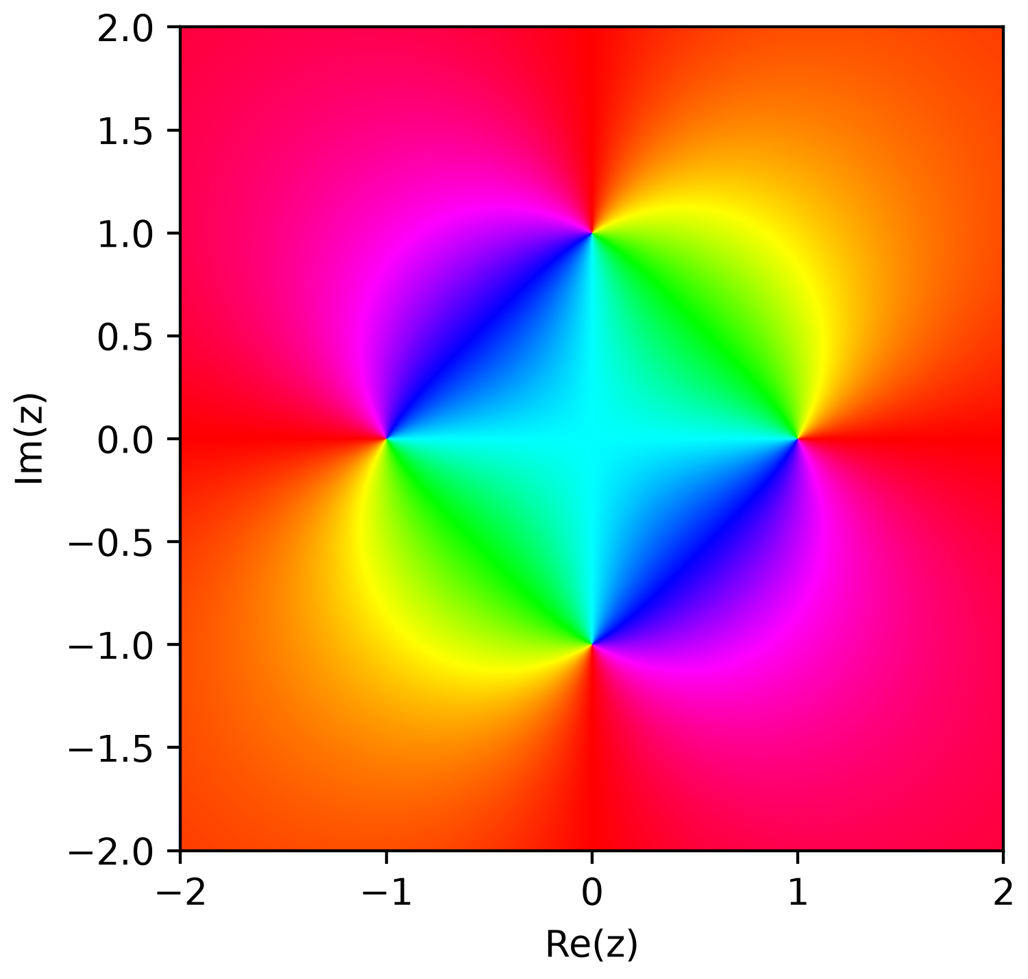
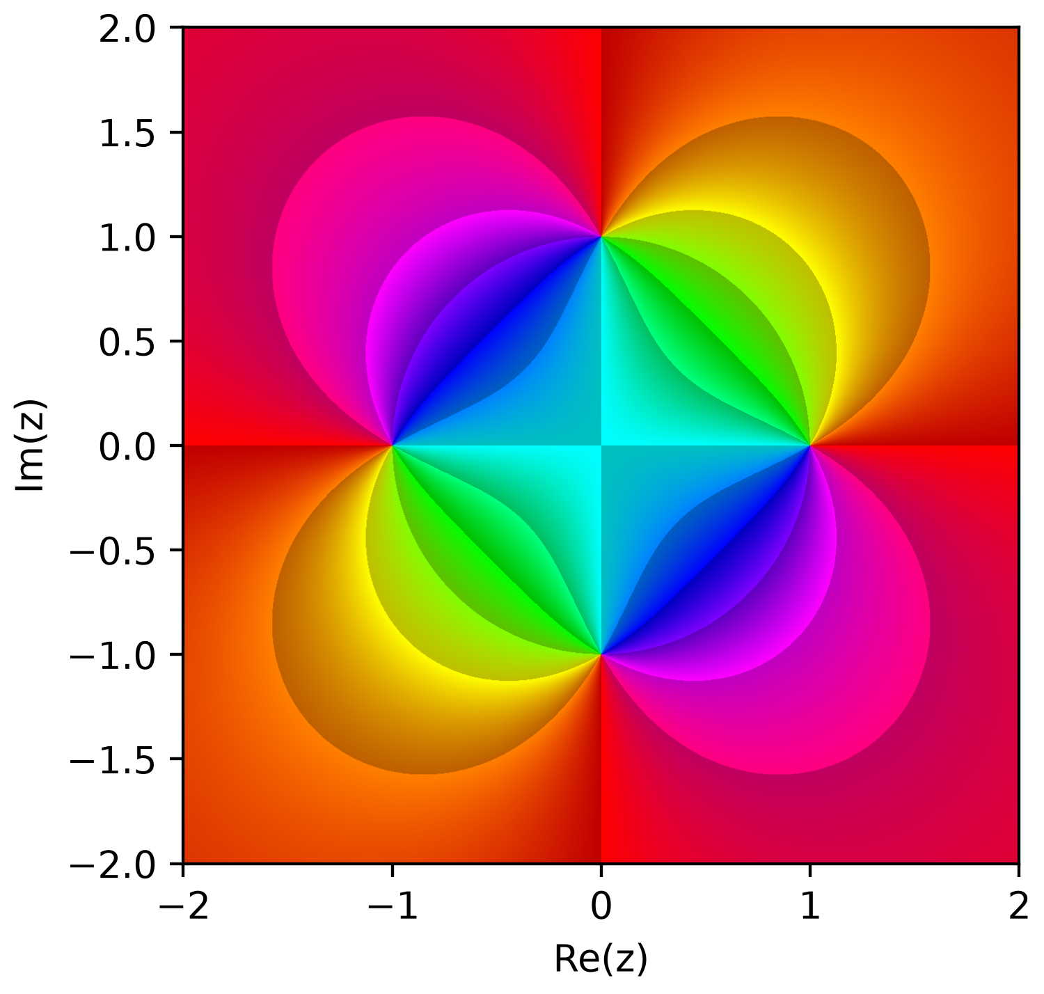
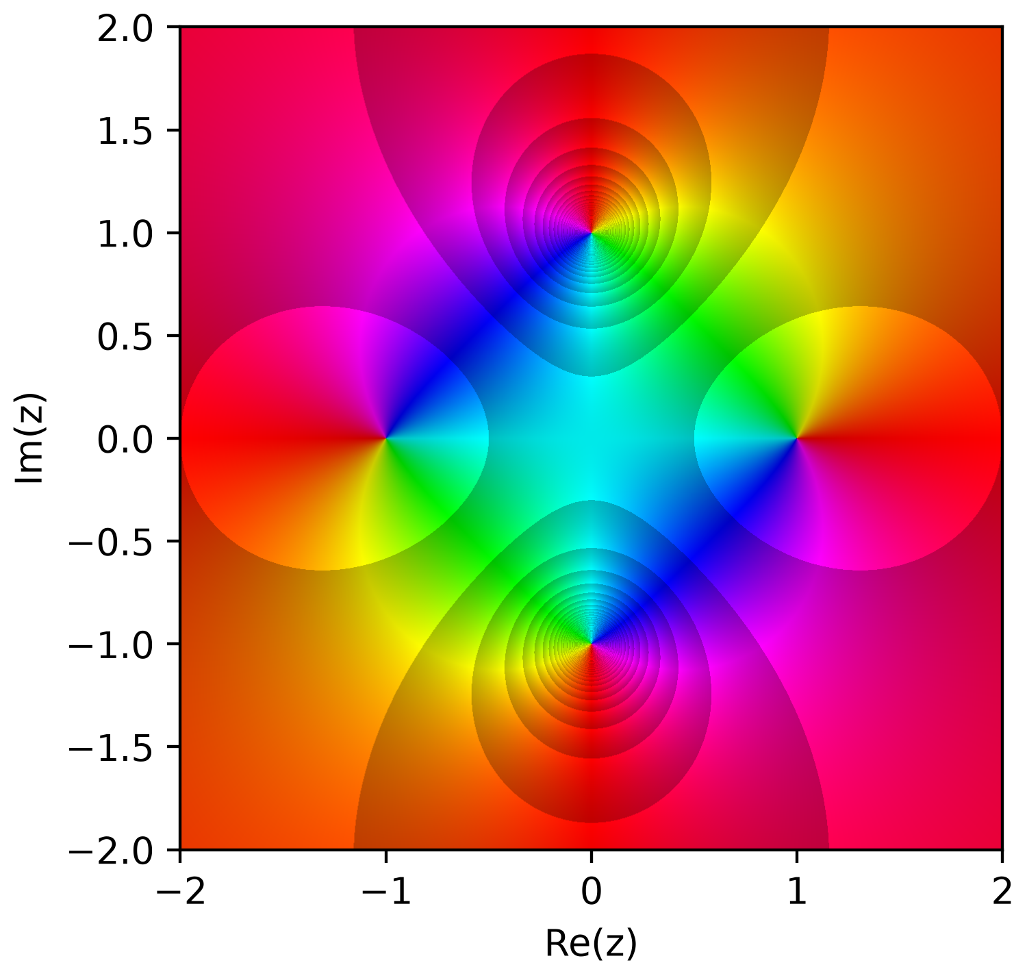
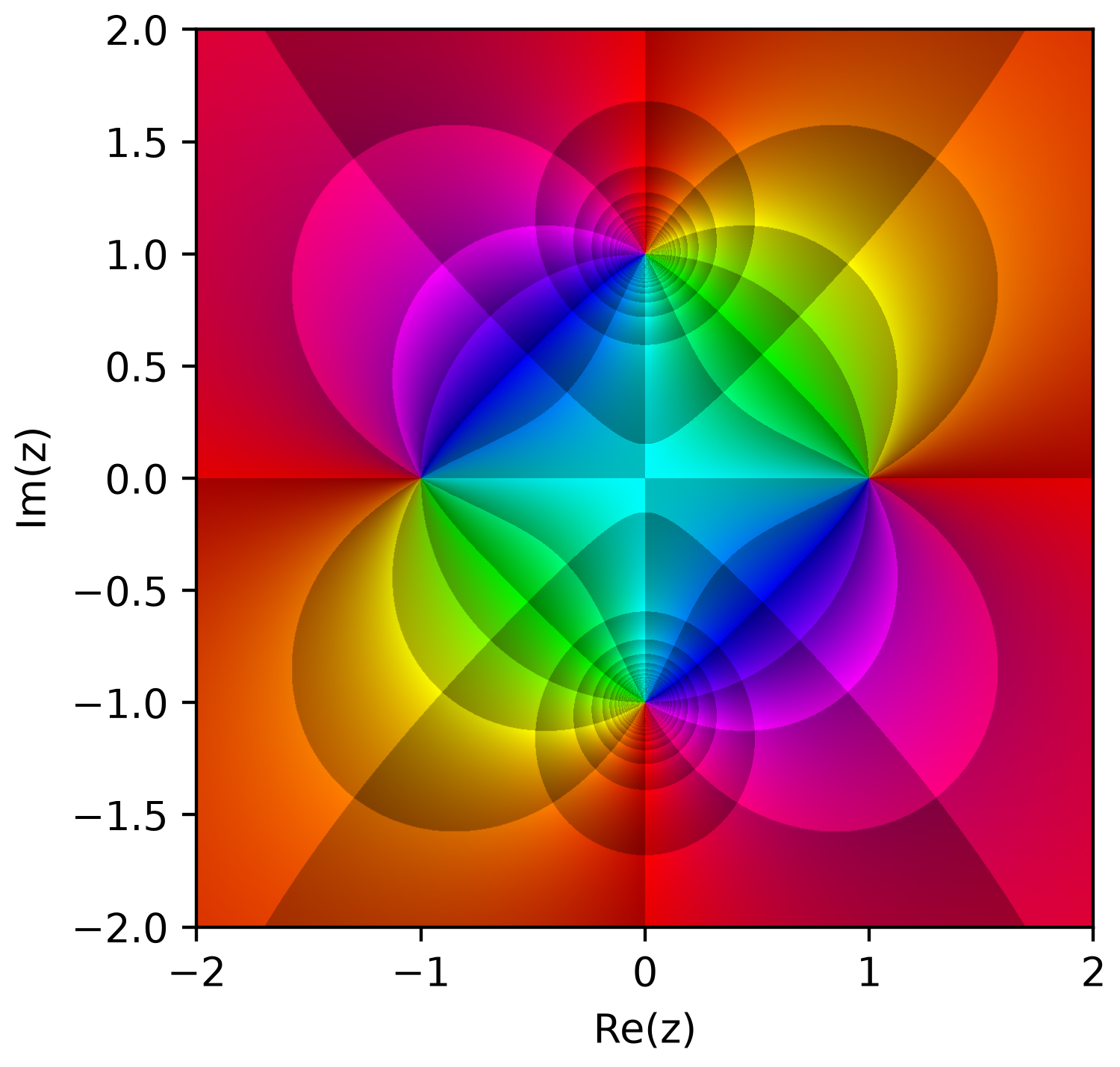
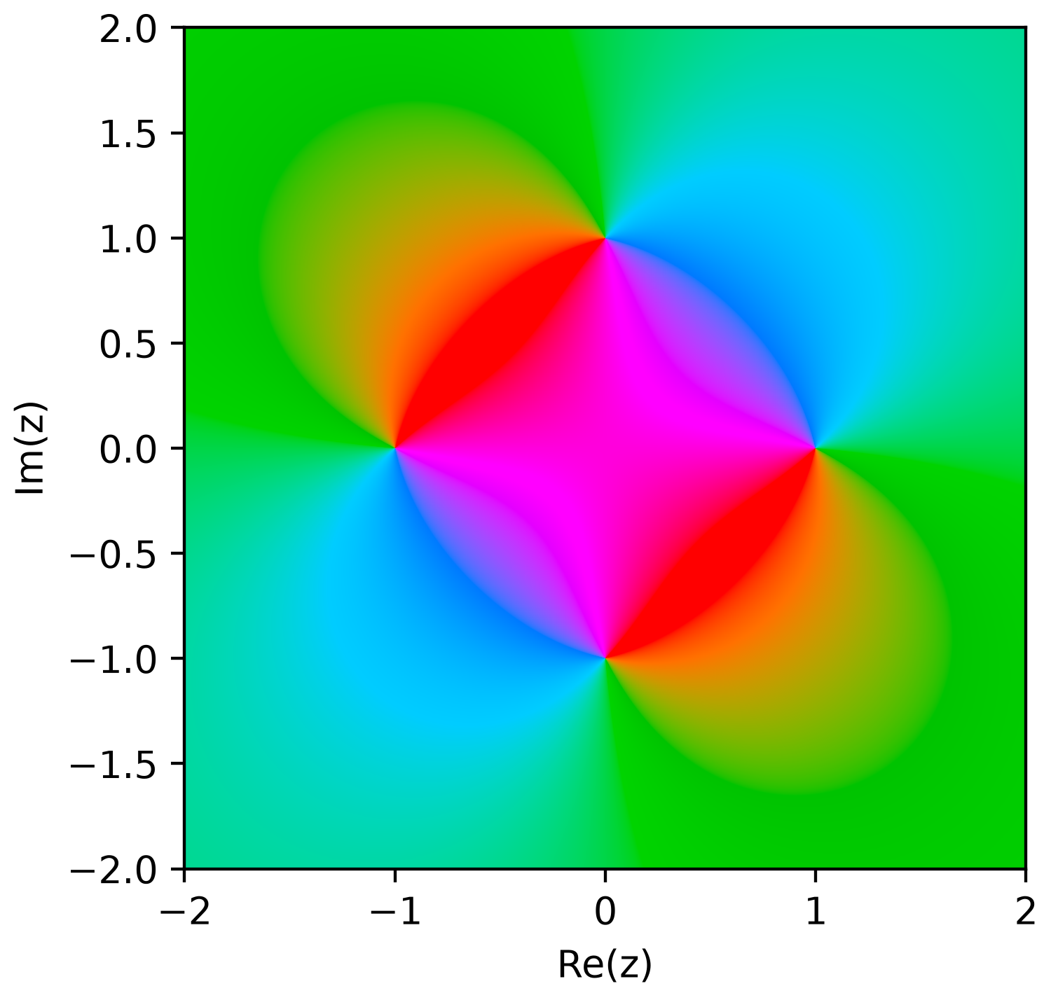
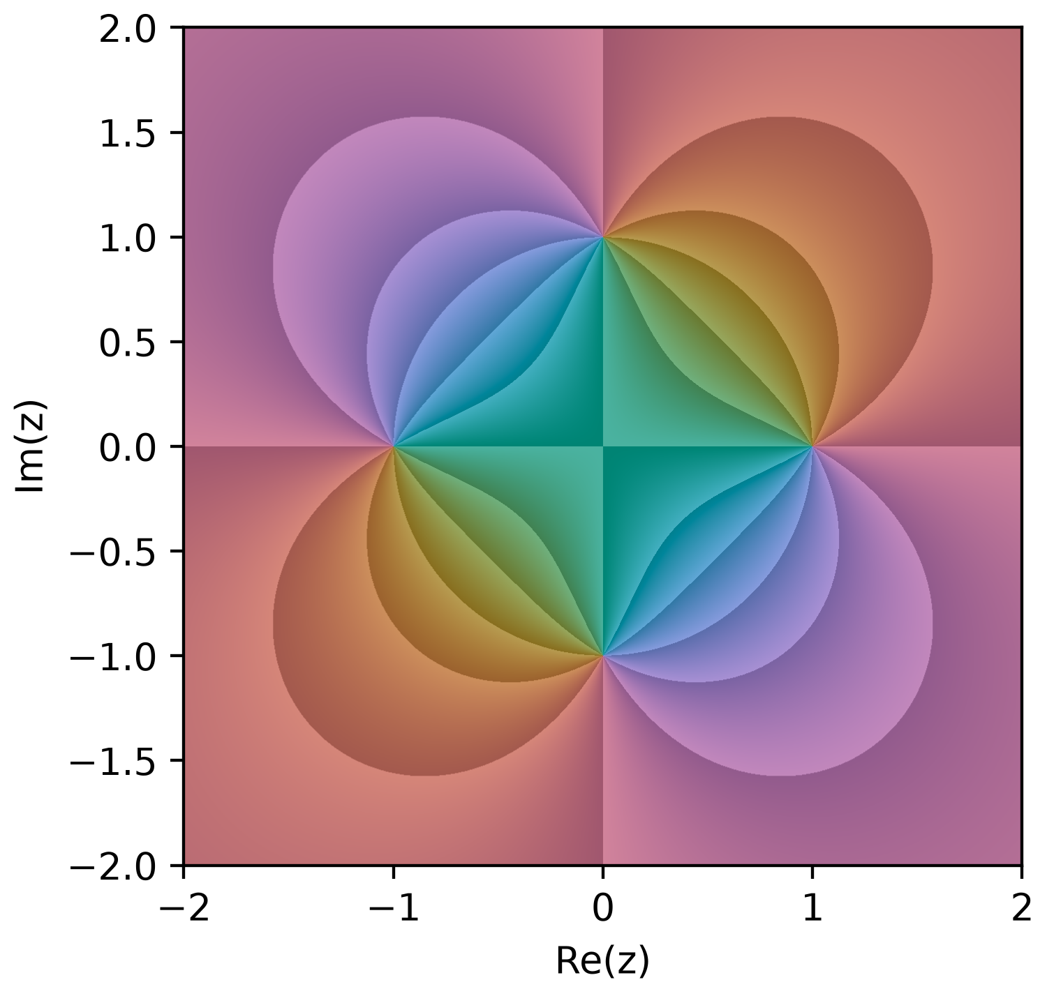
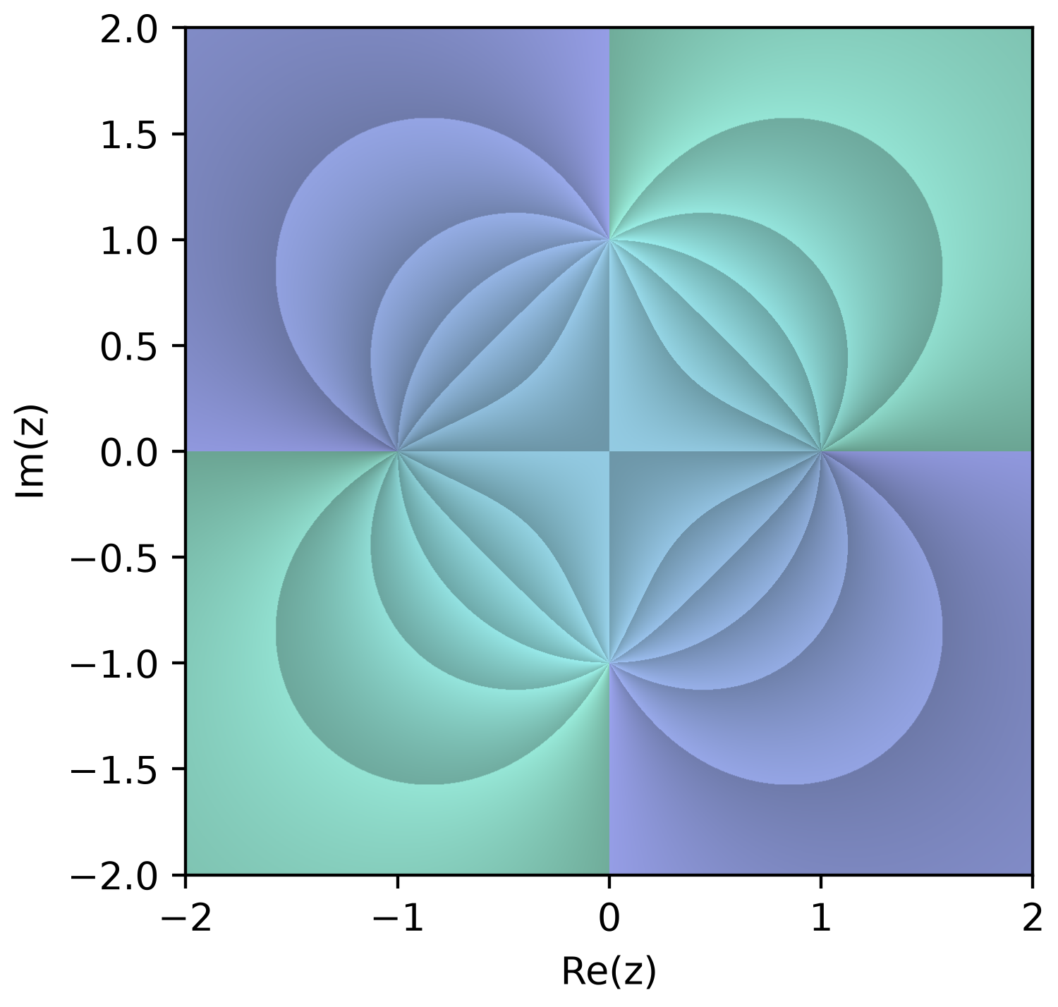
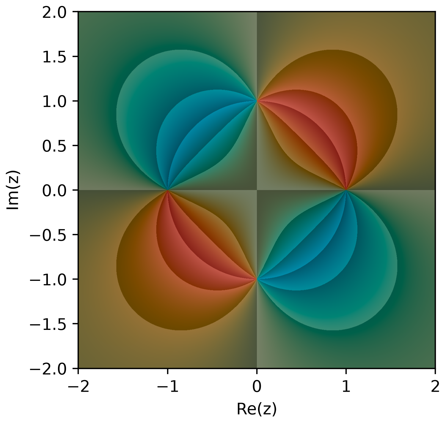
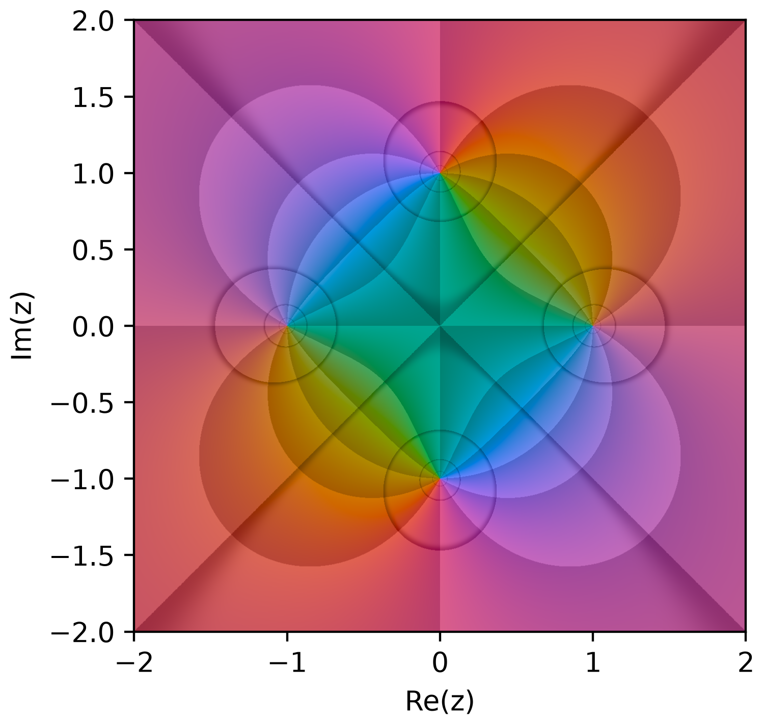
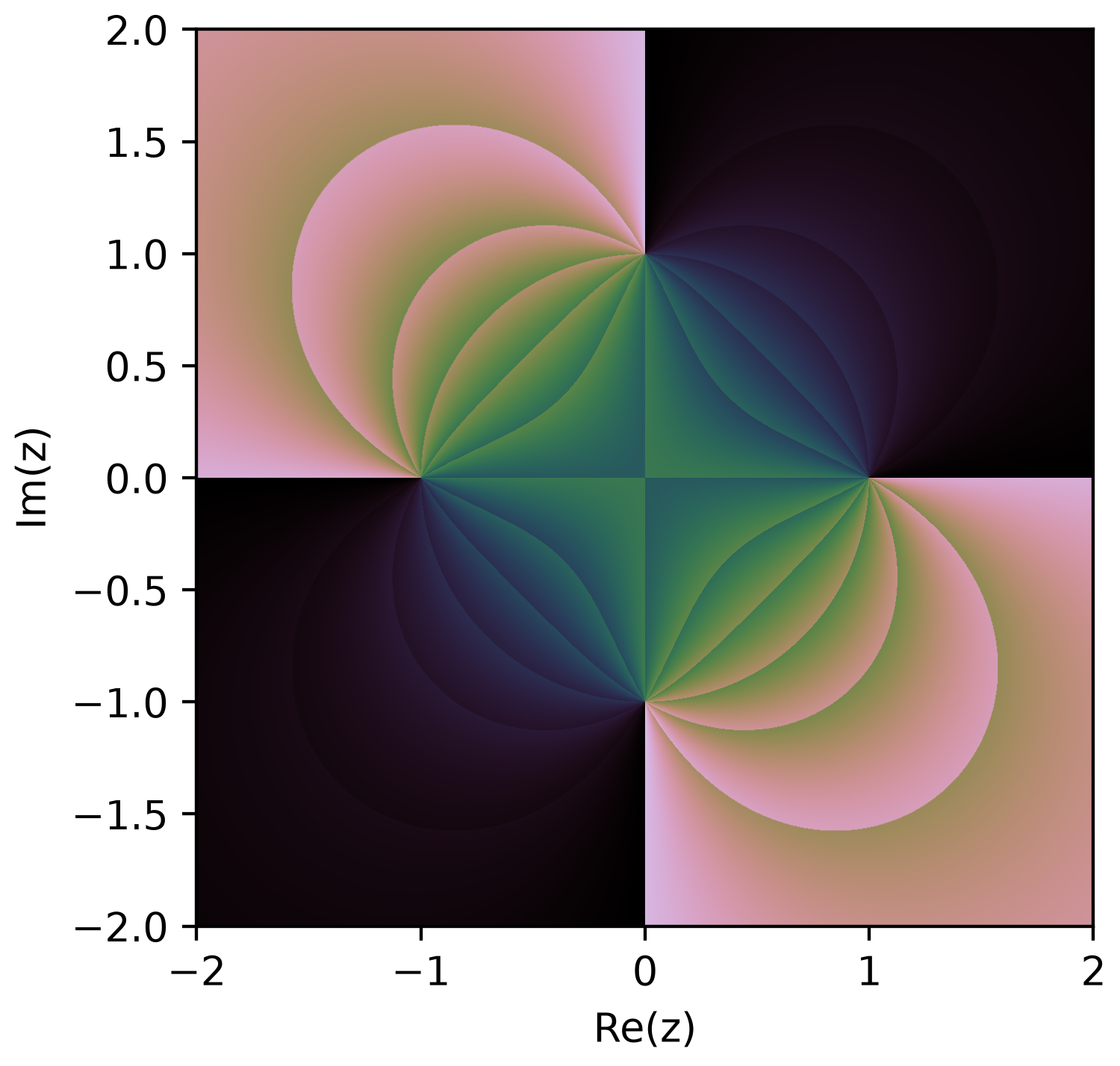
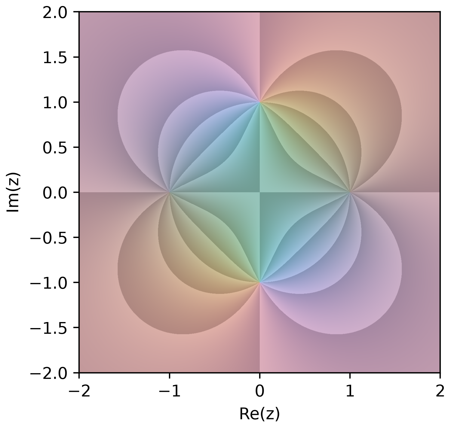
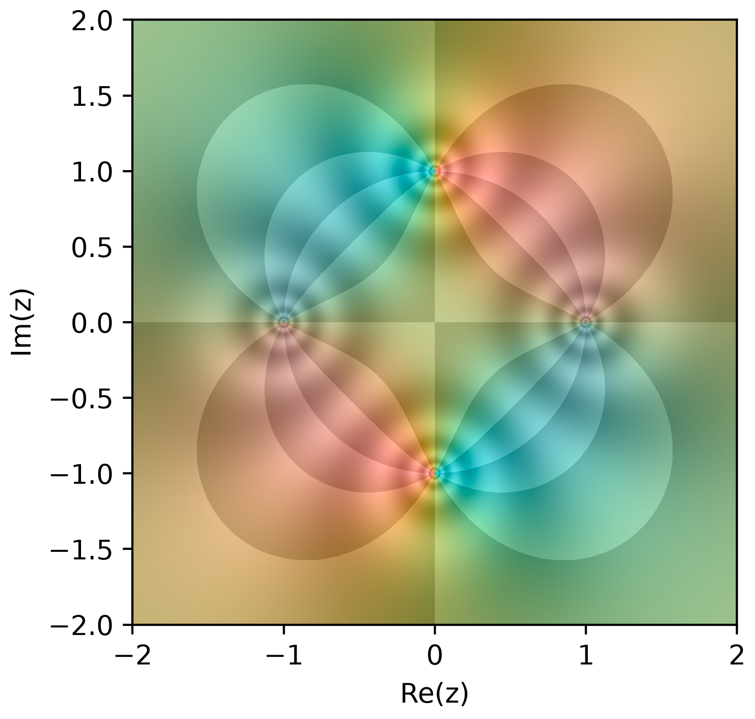
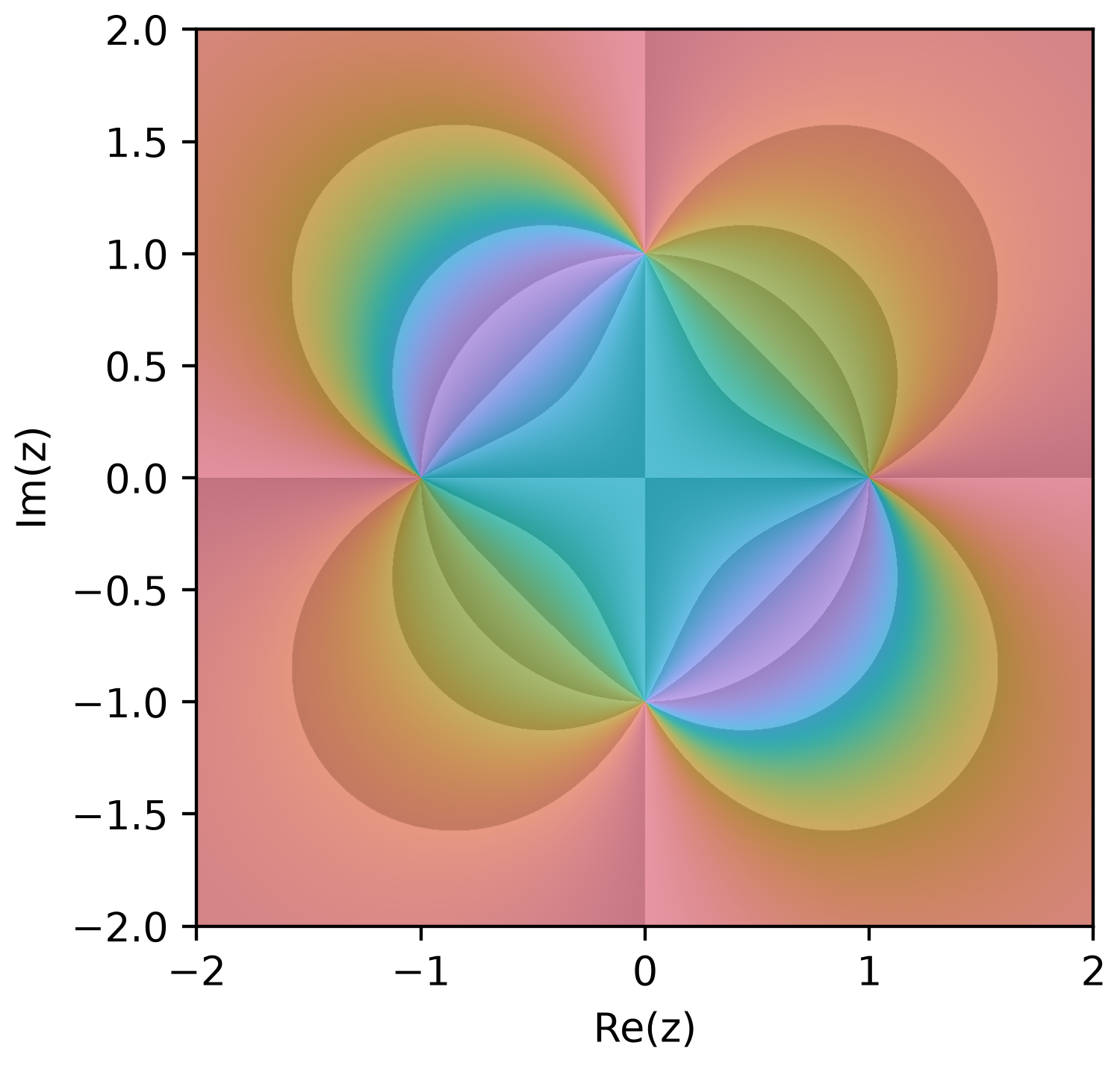
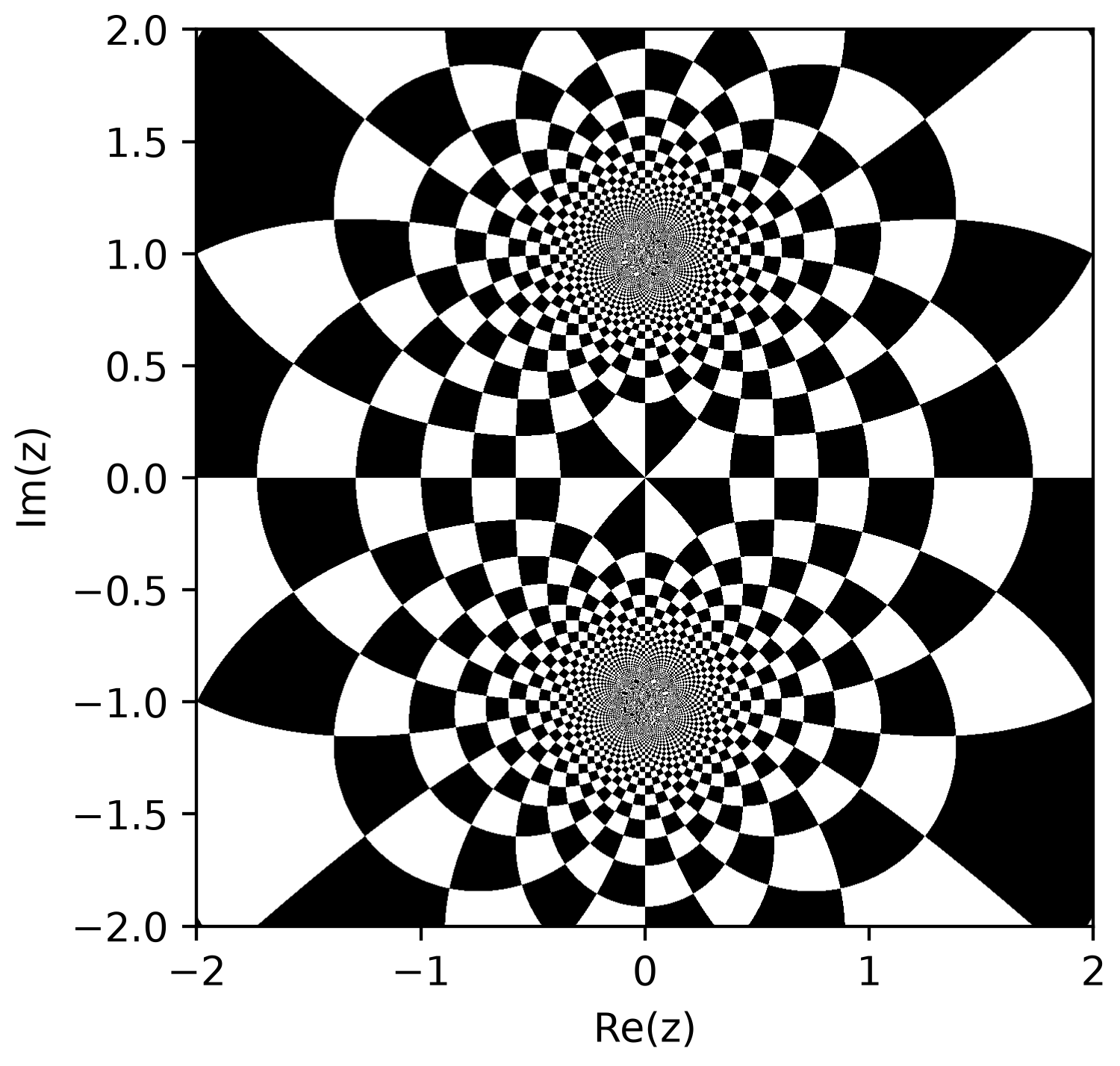
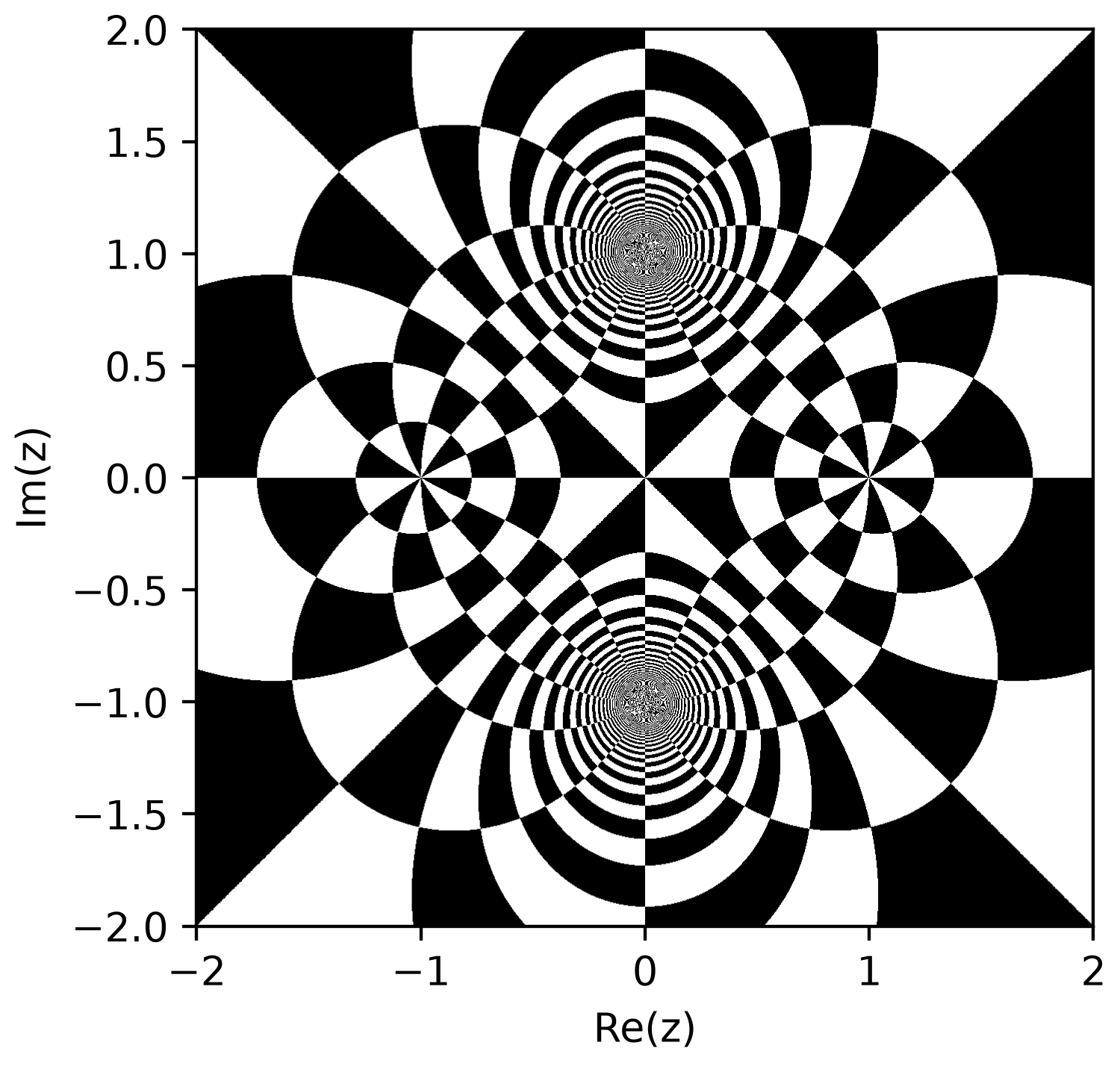
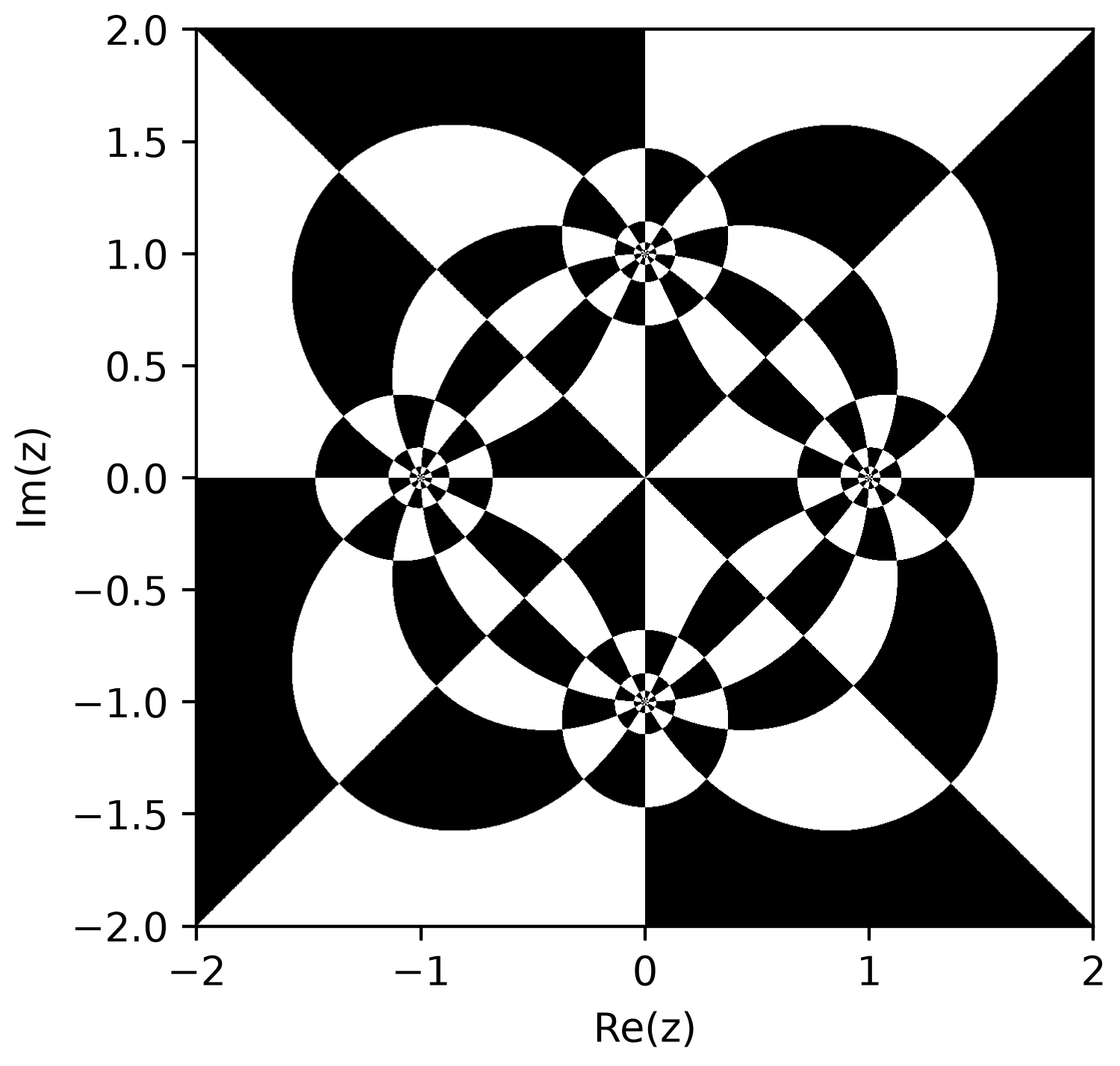
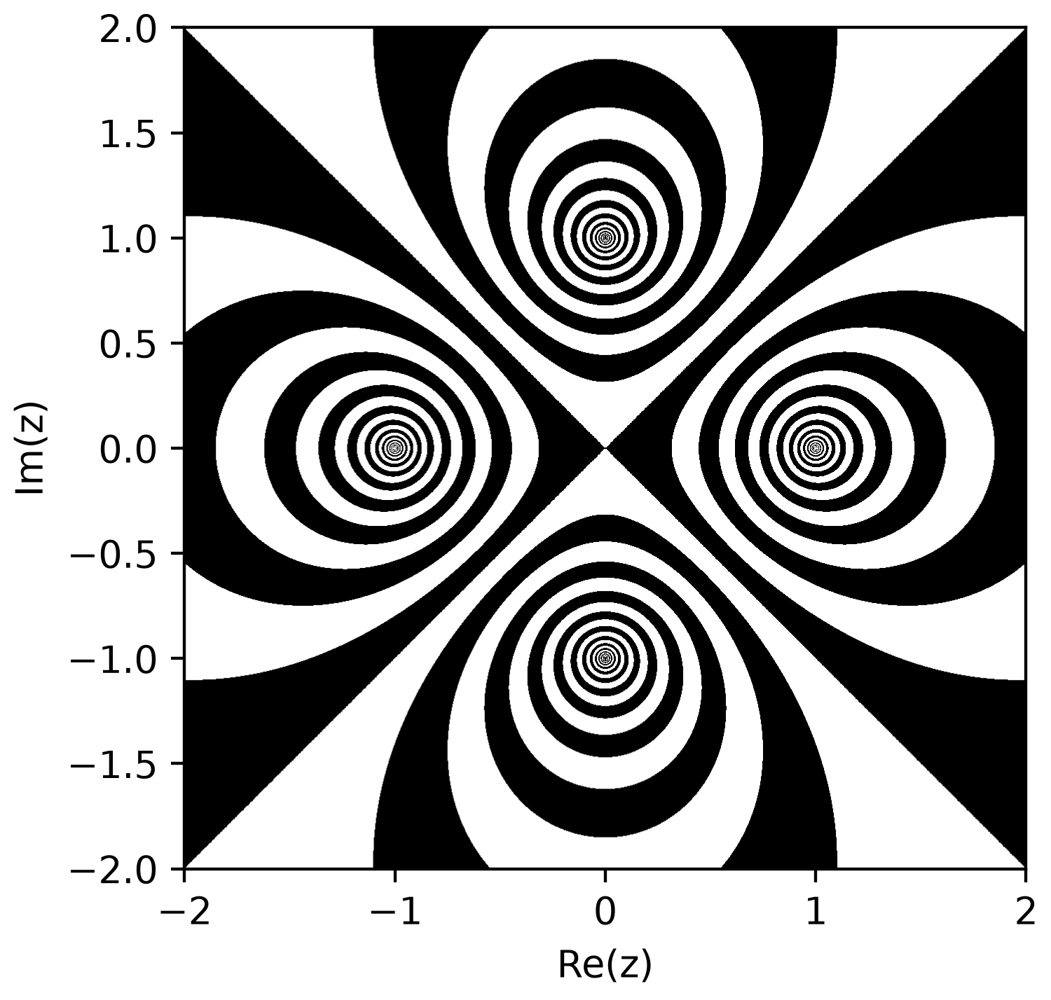
Every colormap on (z2 - 1) / (z2 + 1)
The same function under each colormap the package exports.
Show the code
Physical output
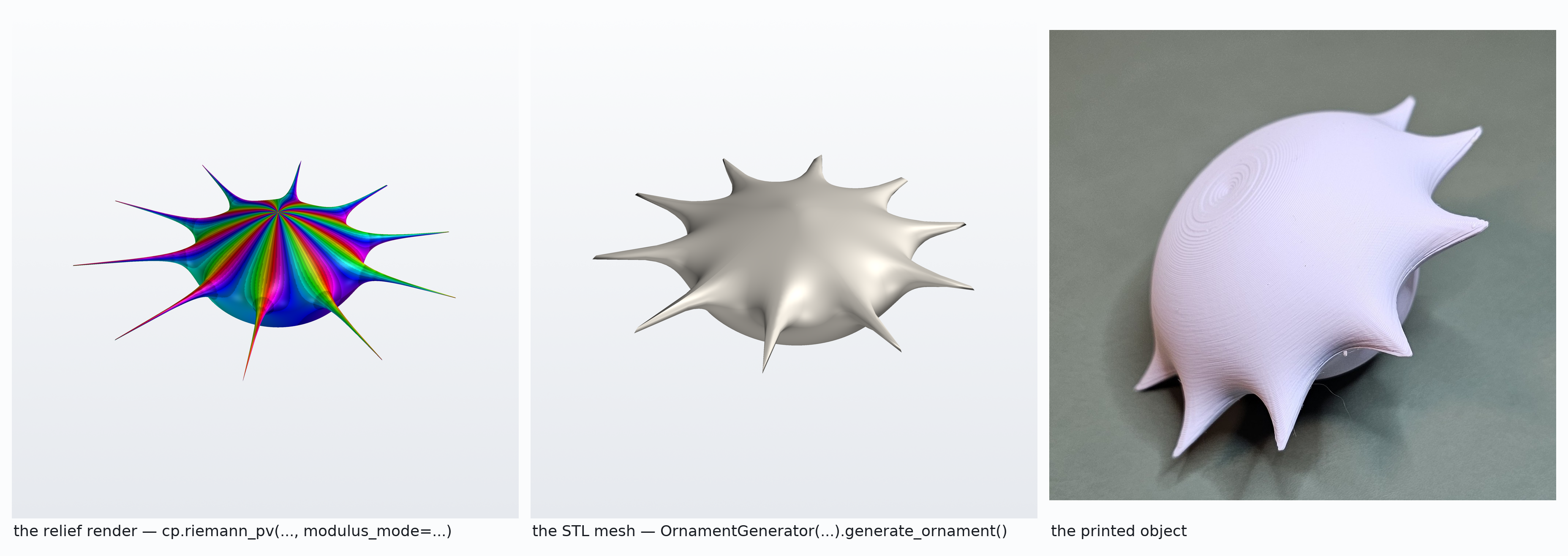
Modulus-scaled relief, exported as a watertight mesh and printed.
From function to printed object
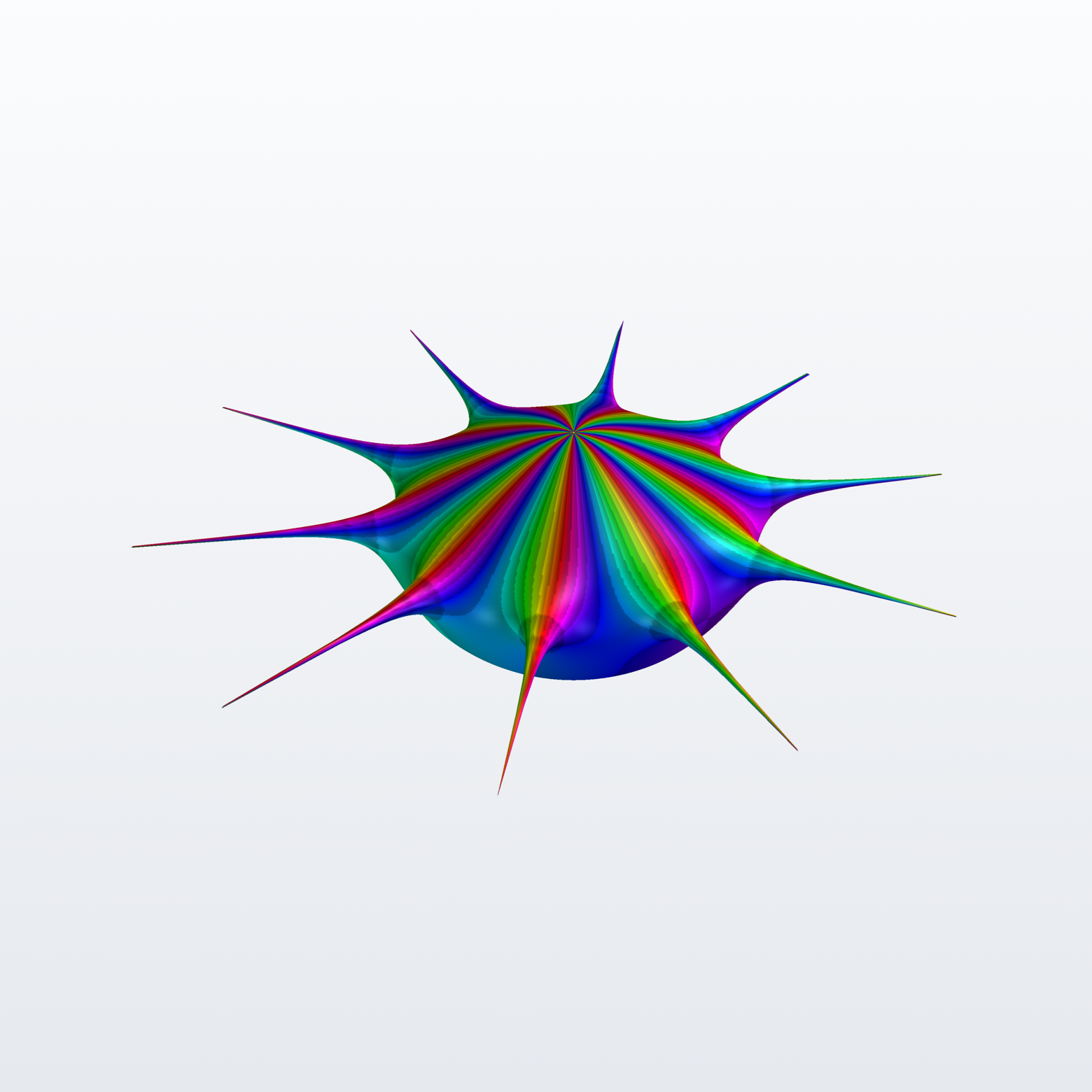
The relief is the mathematics, the mesh is the geometry that survives losing the colour, and the print is the object on a desk. Ten poles become ten spikes around the central zero.
Show the code
import complexplorer as cp
from complexplorer.export.stl import OrnamentGenerator
preset = cp.catalog.get("pole_flower_10")
sc = preset.scaling()
cp.riemann_pv(preset.func, cmap=preset.colormap(),
              modulus_mode=sc["method"], modulus_params=sc["params"])
OrnamentGenerator(preset.func, resolution=150, scaling=sc["method"]).generate_and_save(
    "pole_flower.stl", size_mm=80)
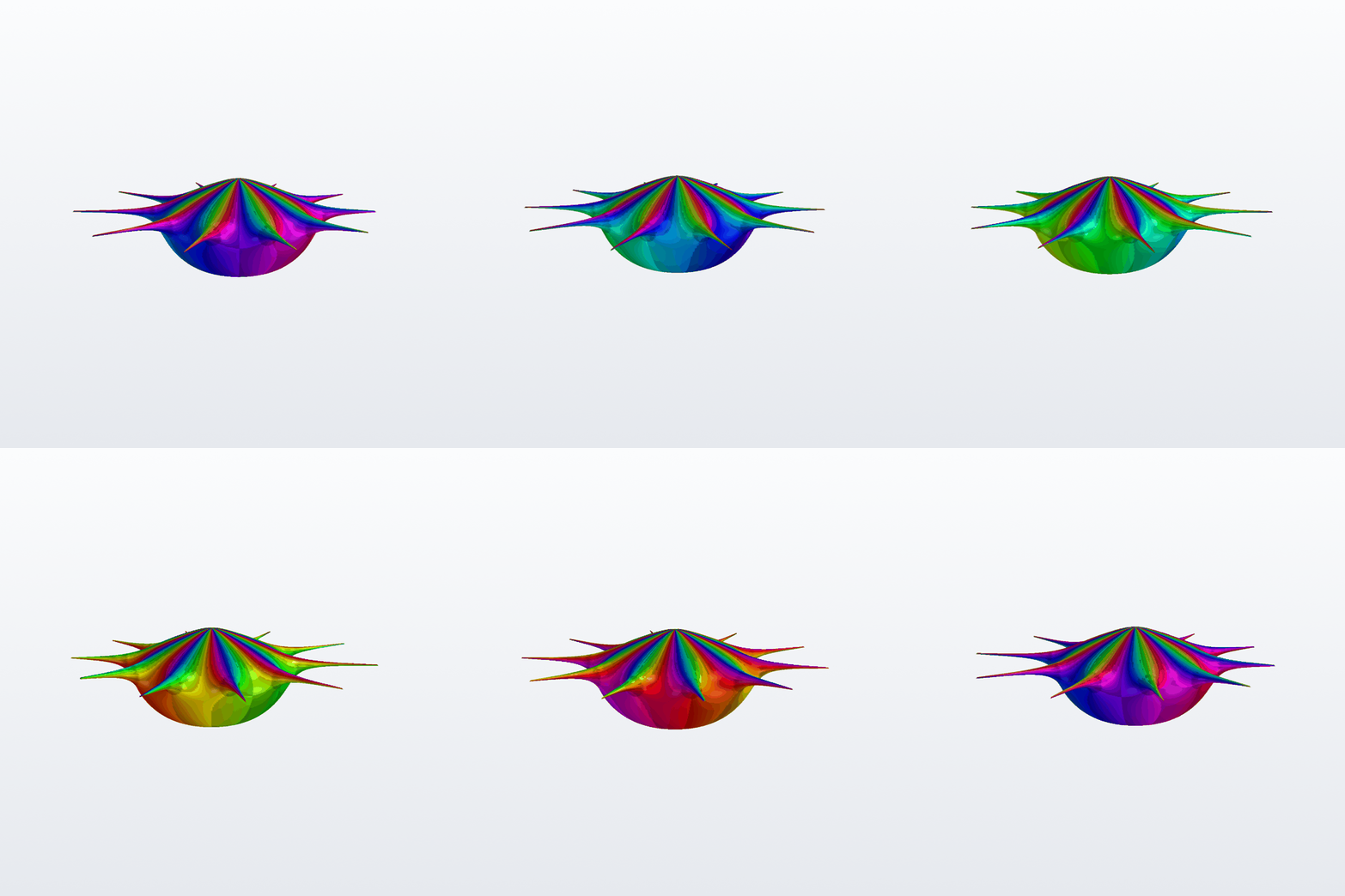
It rotates
A still cannot show depth or how the light moves across the spikes. Every 3D view in the library is an interactive PyVista window; this is 36 frames of one.
Show the code
Cube-Octahedron Dual
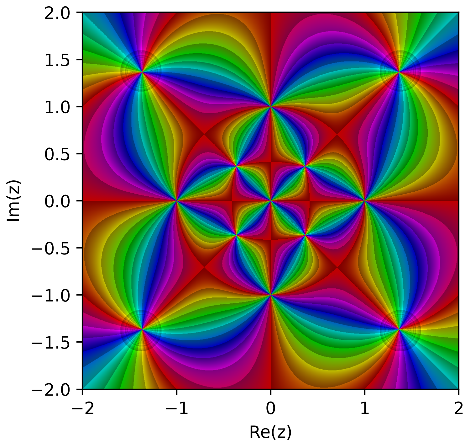
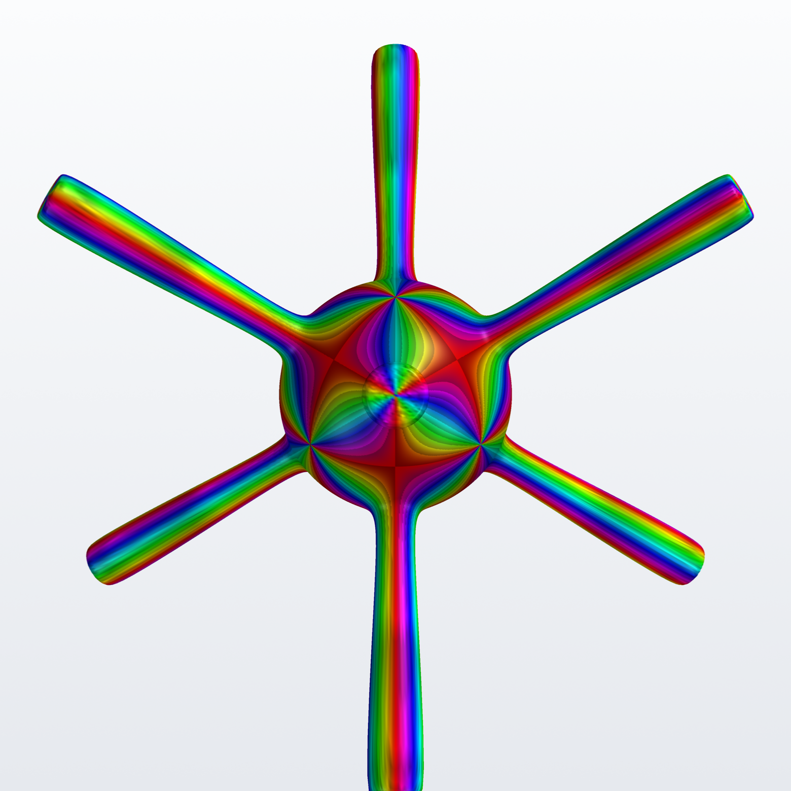
The vertex form of one solid over the vertex form of its dual, at matching binary degree: six order-4 pits on the octahedron's axes, eight triple spikes on the cube's vertices. Full O_h symmetry. Its spikes point along the cube diagonals, which makes it the piece that exposed a sizing bug -- an axis-aligned bounding box understates it by exactly sqrt(3), because each spike projects onto a coordinate axis at 0.577 of its length. One of the six zeros is at infinity, so five are listed.
Show the code
import complexplorer as cp
preset = cp.catalog.get("cube_octahedron_dual")   # f(z) = (z*(z**4 - 1))**4 / (z**8 + 14*z**4 + 1)**3
cp.plot(preset.domain(), preset.func, cmap=preset.colormap())

# ---
import complexplorer as cp
preset = cp.catalog.get("cube_octahedron_dual")   # f(z) = (z*(z**4 - 1))**4 / (z**8 + 14*z**4 + 1)**3
sc = preset.scaling()
cp.riemann_pv(preset.func, cmap=preset.colormap(),
              modulus_mode=sc["method"], modulus_params=sc["params"])  # relief
Dodecahedron-Icosahedron Dual
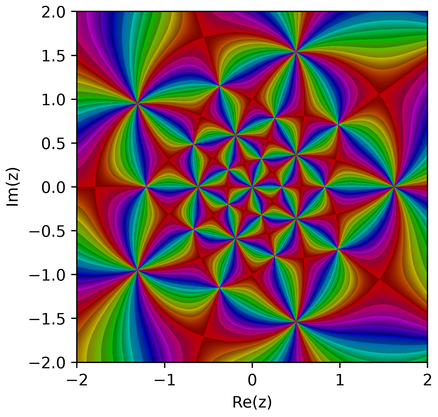
The icosahedral twin of the Cube-Octahedron Dual, built the same way: one solid's vertex form over its dual's, at matching degree. Twenty triple spikes on the dodecahedron's vertices, twelve order-5 pits on the icosahedron's. Its spikes sit exactly where the Icosahedral Crown has its pits. Full I_h symmetry. One zero is at infinity; eleven are listed.
Show the code
import complexplorer as cp
preset = cp.catalog.get("dodecahedron_icosahedron_dual")   # f(z) = (z*(z**10 - 11*z**5 - 1))**5 / (z**20 + 228*z**15 + 494*z**10 - 228*z**5 + 1)**3
cp.plot(preset.domain(), preset.func, cmap=preset.colormap())

# ---
import complexplorer as cp
preset = cp.catalog.get("dodecahedron_icosahedron_dual")   # f(z) = (z*(z**10 - 11*z**5 - 1))**5 / (z**20 + 228*z**15 + 494*z**10 - 228*z**5 + 1)**3
sc = preset.scaling()
cp.riemann_pv(preset.func, cmap=preset.colormap(),
              modulus_mode=sc["method"], modulus_params=sc["params"])  # relief
Icosahedral Crown
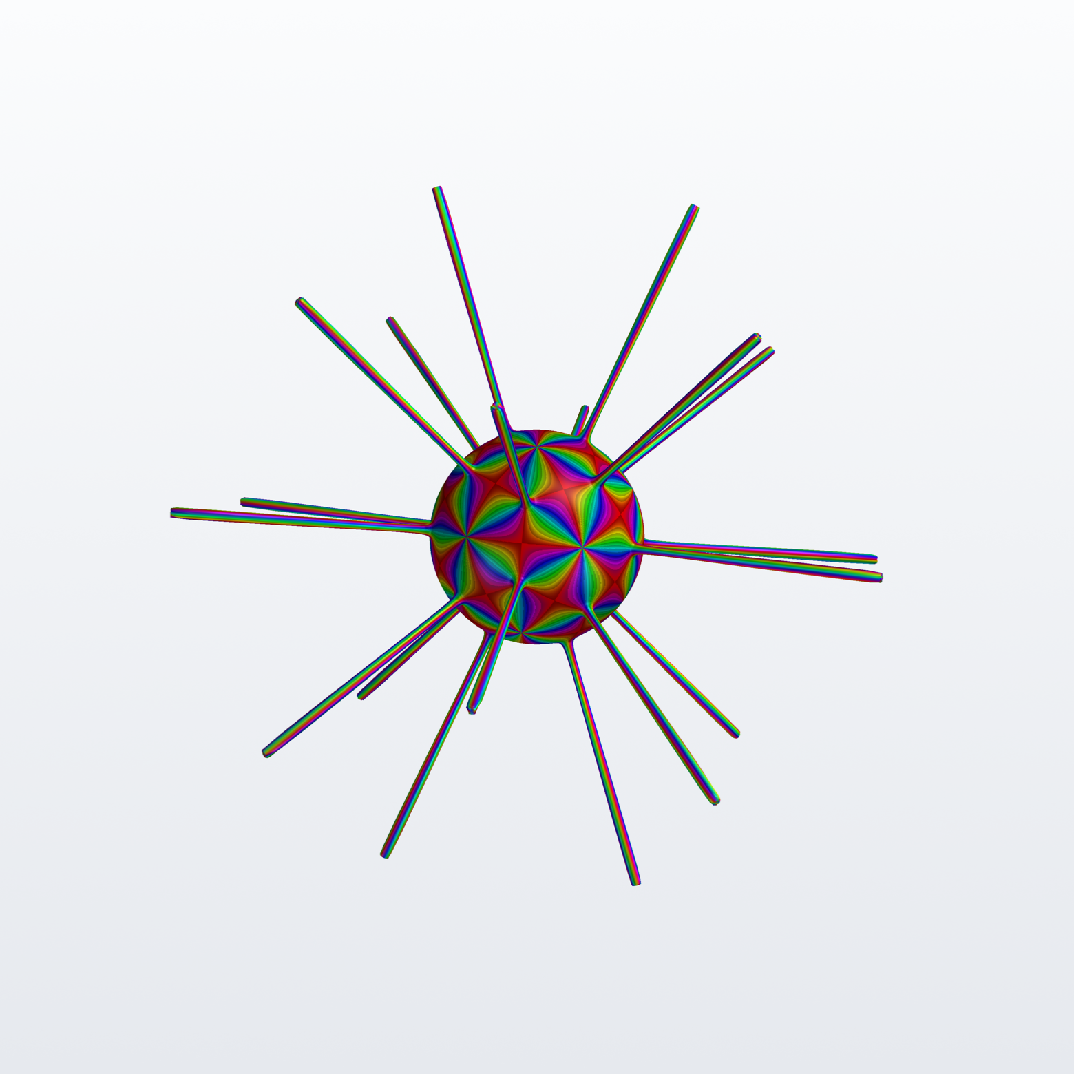
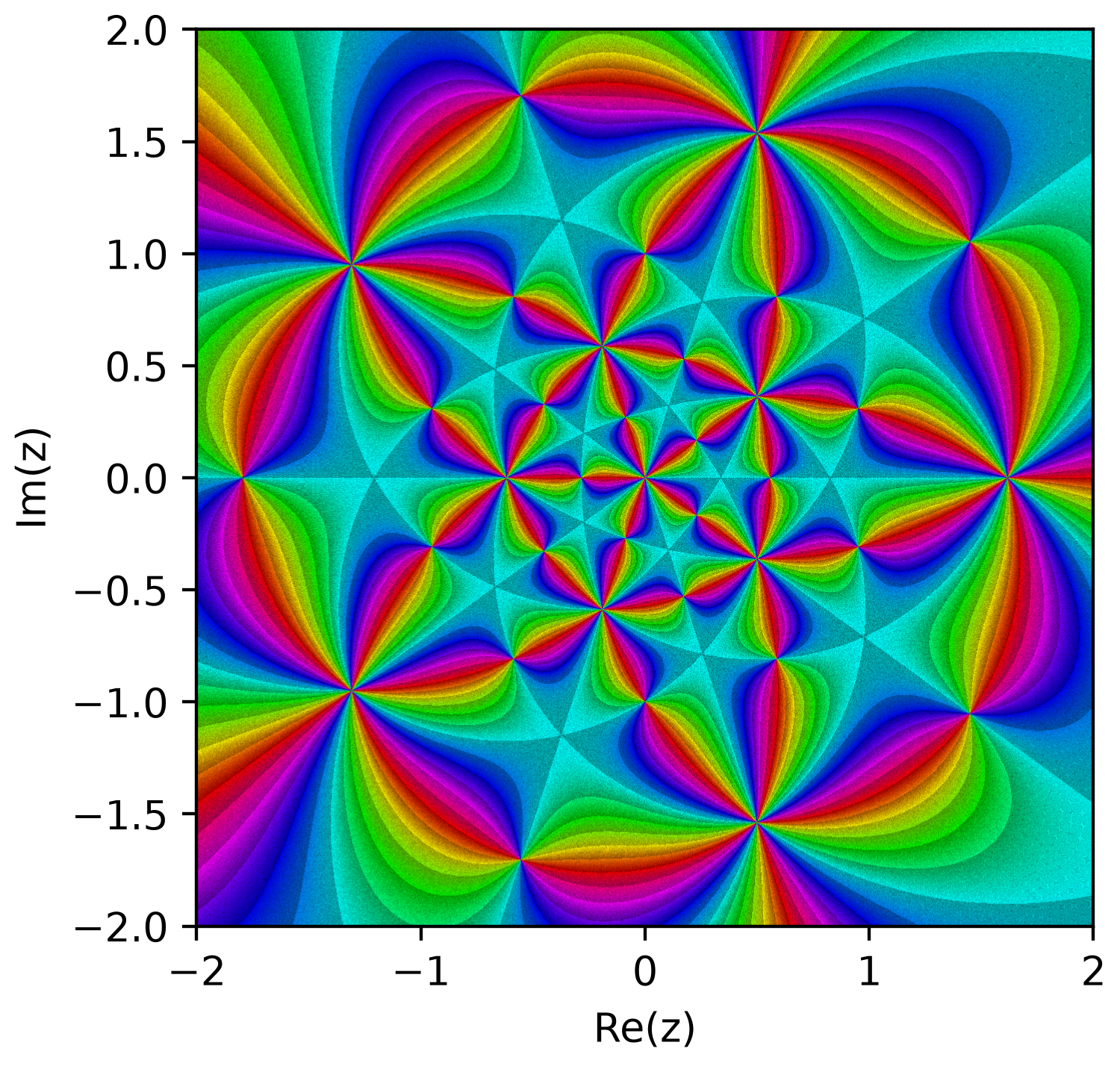
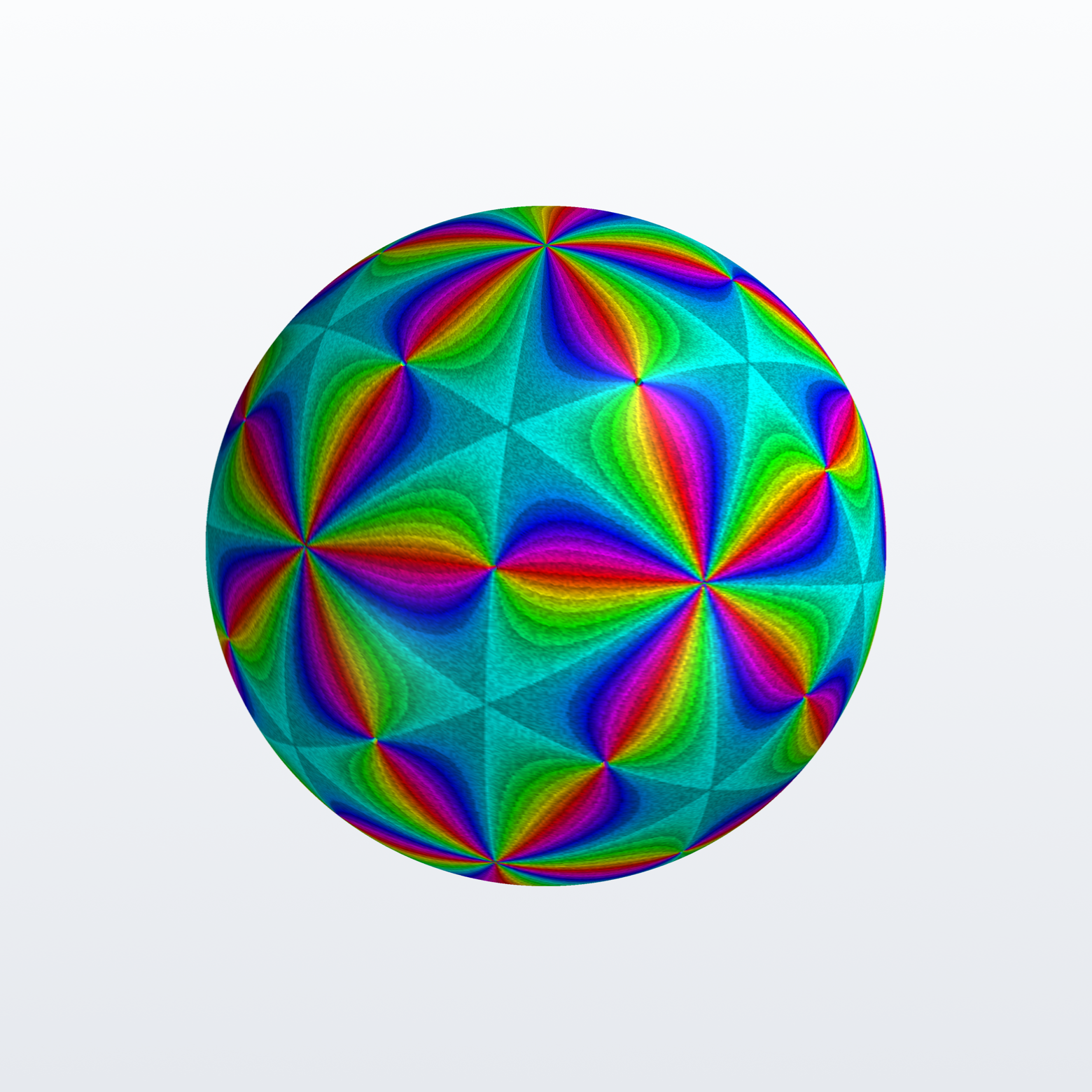
The icosahedral answer to the Octahedral Crown, and a jump from binary degree 12 to 60 -- the icosahedral rotation group has order 60, so 60 is the lowest degree any invariant ratio can have. Twelve spikes of order 5 at the icosahedron's vertices over thirty double pits at its edge midpoints. Full I_h symmetry (order 120), the largest here. Its features are order 5, so the derived transfer scale is capped: this is the piece the cap exists for, because a mesh cannot deliver the dynamic range an uncapped order-5 scale asks for. One pole is at infinity; eleven are listed.
Show the code
import complexplorer as cp
preset = cp.catalog.get("icosahedral_crown")   # f(z) = (z**30 - 522*z**25 - 10005*z**20 - 10005*z**10 + 522*z**5 + 1)**2 / (z*(z**10 - 11*z**5 - 1))**5
cp.plot(preset.domain(), preset.func, cmap=preset.colormap())

# ---
import complexplorer as cp
preset = cp.catalog.get("icosahedral_crown")   # f(z) = (z**30 - 522*z**25 - 10005*z**20 - 10005*z**10 + 522*z**5 + 1)**2 / (z*(z**10 - 11*z**5 - 1))**5
sc = preset.scaling()
cp.riemann_pv(preset.func, cmap=preset.colormap(),
              modulus_mode=sc["method"], modulus_params=sc["params"])  # relief
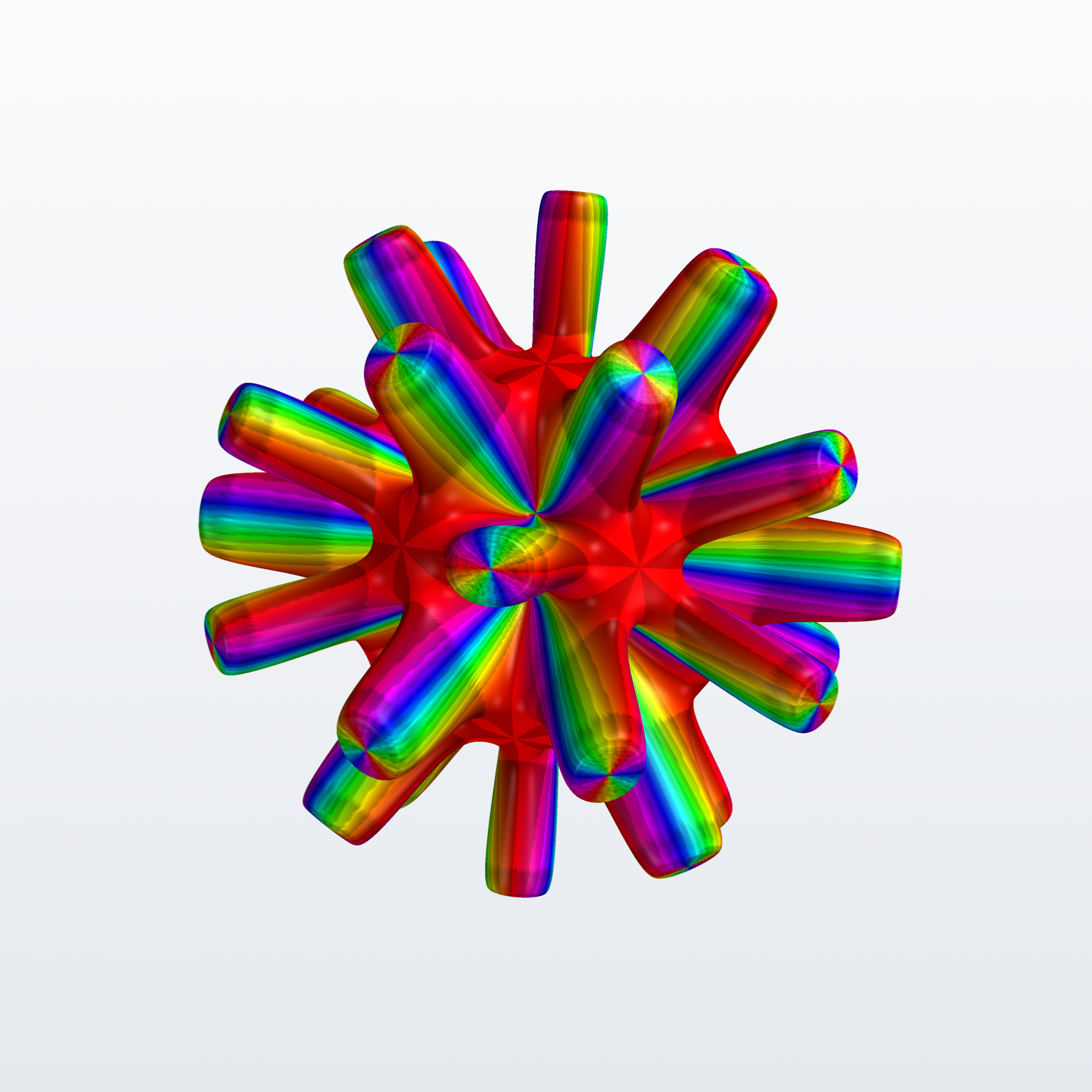
Icosidodecahedral Star
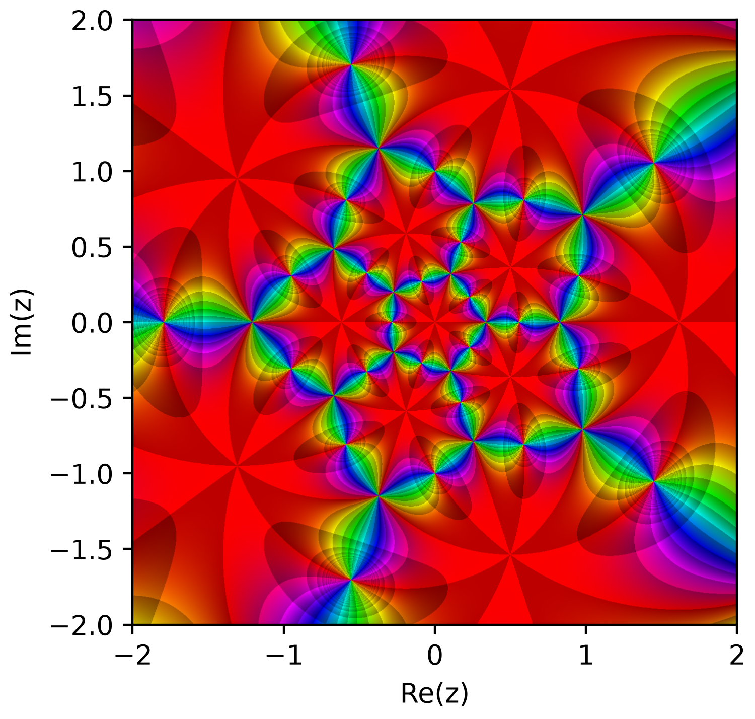
The third degree-60 icosahedral ratio, and the one with no counterpart elsewhere in the family: thirty double spikes at the icosahedron's edge midpoints -- the vertices of an icosidodecahedron -- over twenty triple pits on the dodecahedron. The densest piece here, and the most sea-urchin-like. Full I_h symmetry, and no feature at infinity: both forms are full degree, so the answer key is complete.
Show the code
import complexplorer as cp
preset = cp.catalog.get("icosidodecahedral_star")   # f(z) = (z**20 + 228*z**15 + 494*z**10 - 228*z**5 + 1)**3 / (z**30 - 522*z**25 - 10005*z**20 - 10005*z**10 + 522*z**5 + 1)**2
cp.plot(preset.domain(), preset.func, cmap=preset.colormap())

# ---
import complexplorer as cp
preset = cp.catalog.get("icosidodecahedral_star")   # f(z) = (z**20 + 228*z**15 + 494*z**10 - 228*z**5 + 1)**3 / (z**30 - 522*z**25 - 10005*z**20 - 10005*z**10 + 522*z**5 + 1)**2
sc = preset.scaling()
cp.riemann_pv(preset.func, cmap=preset.colormap(),
              modulus_mode=sc["method"], modulus_params=sc["params"])  # relief
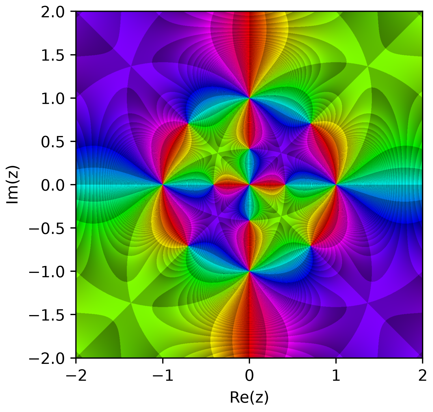
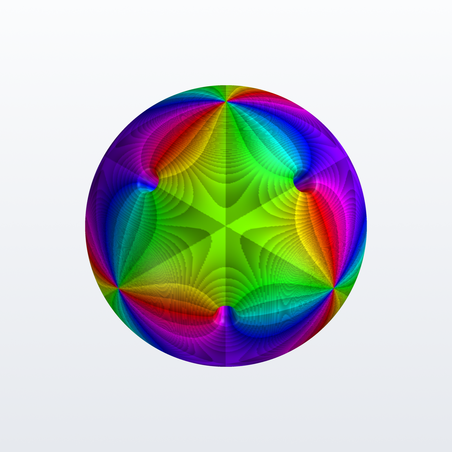
Octahedral Crown
Twelve simple zeros at the octahedron's edge midpoints under six double poles at its vertices: a crown of six spikes with a pit between each neighbouring pair. Full O_h symmetry (order 48, all nine mirror planes), so any coordinate plane cuts it into identical halves. The sixth pole sits at the north pole of the sphere, i.e. at infinity, so the answer key below lists five of the six.
Show the code
import complexplorer as cp
preset = cp.catalog.get("octahedral_crown")   # f(z) = (z**12 - 33*z**8 - 33*z**4 + 1) / (z*(z**4 - 1))**2
cp.plot(preset.domain(), preset.func, cmap=preset.colormap())

# ---
import complexplorer as cp
preset = cp.catalog.get("octahedral_crown")   # f(z) = (z**12 - 33*z**8 - 33*z**4 + 1) / (z*(z**4 - 1))**2
sc = preset.scaling()
cp.riemann_pv(preset.func, cmap=preset.colormap(),
              modulus_mode=sc["method"], modulus_params=sc["params"])  # relief
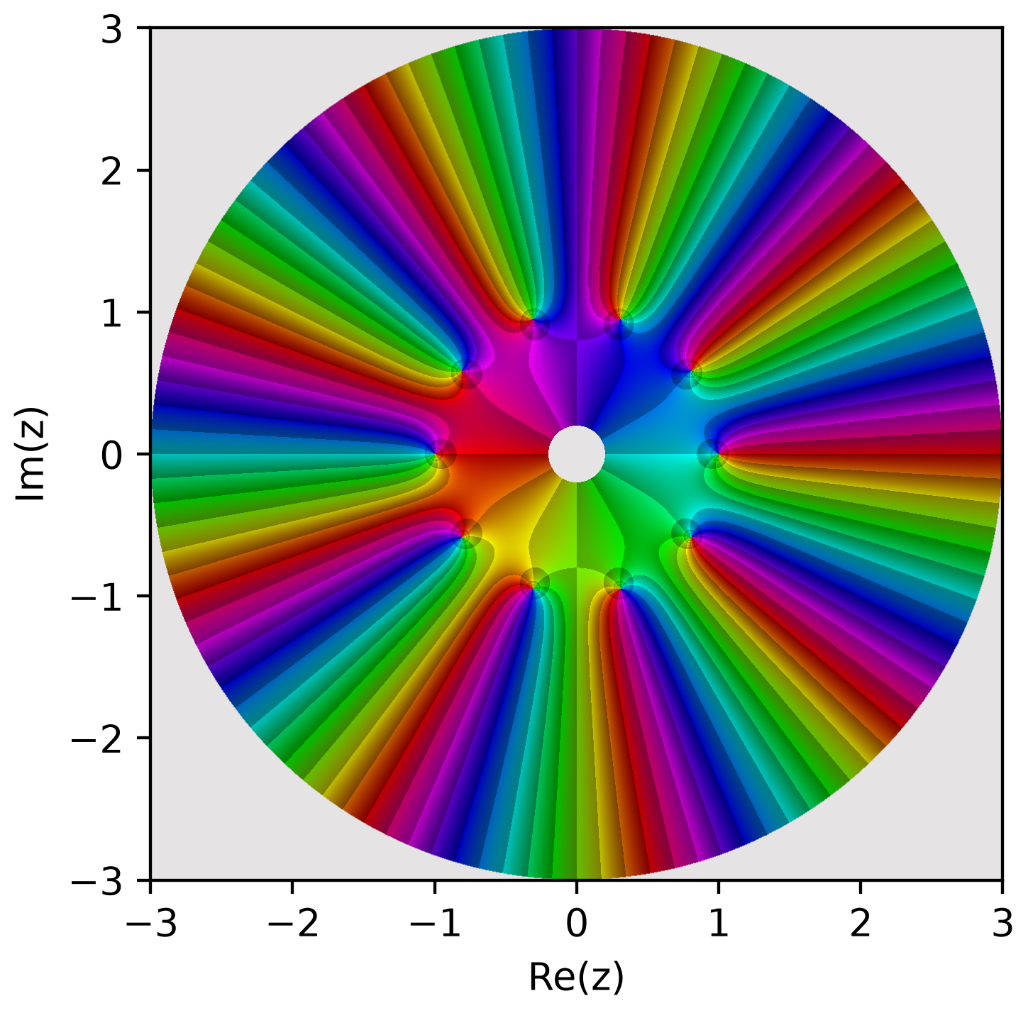
Pole Flower 10
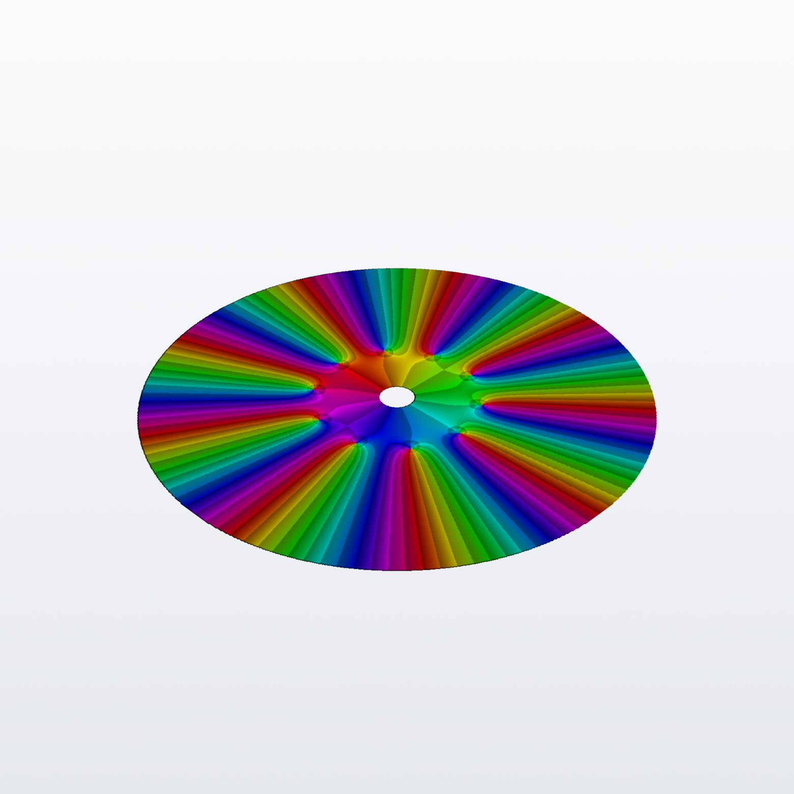
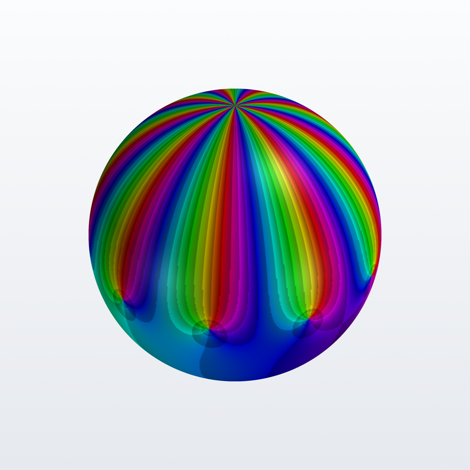
A ring of ten simple poles (the 10th roots of unity) around a central simple zero. The signature printable ornament.
Show the code
import complexplorer as cp
preset = cp.catalog.get("pole_flower_10")   # f(z) = z / (z**10 - 1)
cp.plot(preset.domain(), preset.func, cmap=preset.colormap())

# ---
import complexplorer as cp
preset = cp.catalog.get("pole_flower_10")   # f(z) = z / (z**10 - 1)
sc = preset.scaling()
cp.riemann_pv(preset.func, cmap=preset.colormap(),
              modulus_mode=sc["method"], modulus_params=sc["params"])  # relief

# ---
import complexplorer as cp
preset = cp.catalog.get("pole_flower_10")   # f(z) = z / (z**10 - 1)
sc = preset.scaling()
cp.plot_landscape_pv(preset.domain(), preset.func, cmap=preset.colormap(),
                     modulus_mode=sc["method"], modulus_params=sc["params"])

# ---
import complexplorer as cp
preset = cp.catalog.get("pole_flower_10")   # f(z) = z / (z**10 - 1)
cp.riemann_pv(preset.func, cmap=preset.colormap())   # full sphere
Tetrahedral Dual
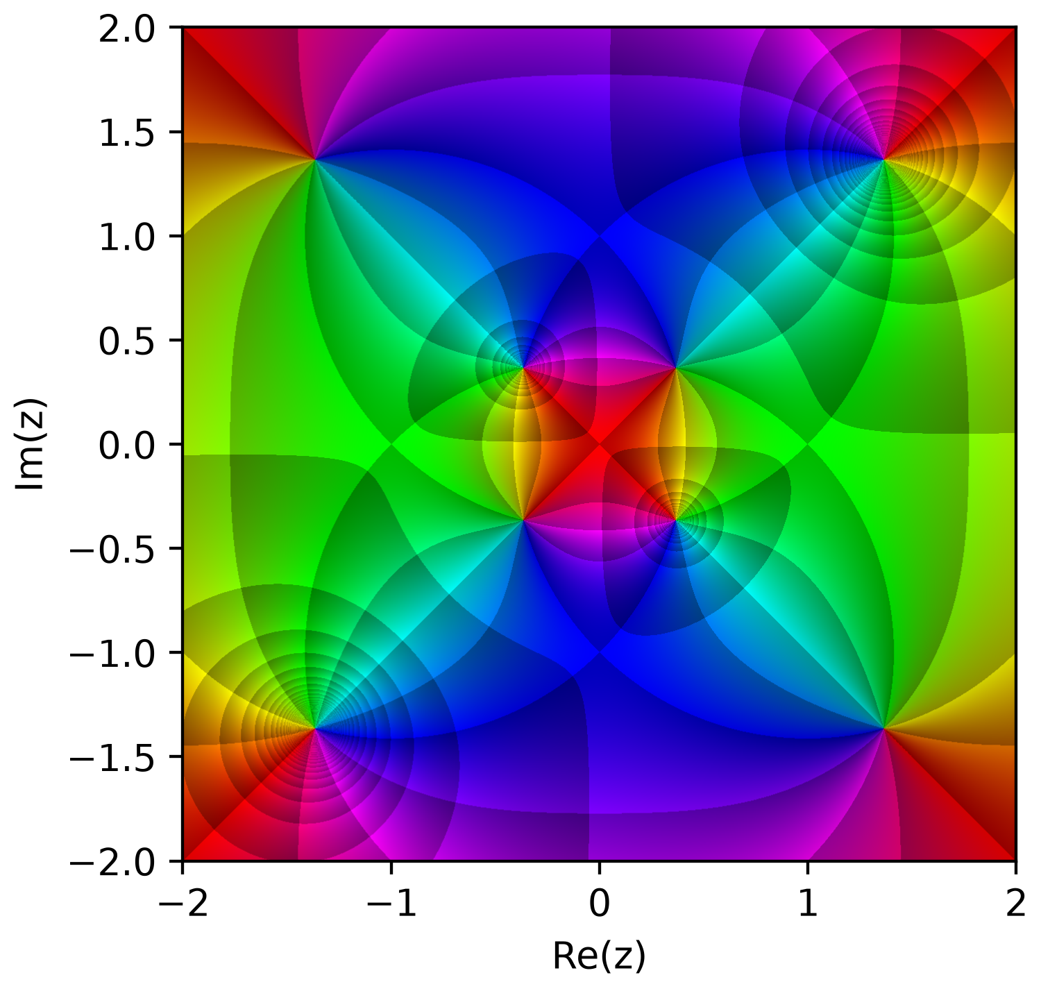
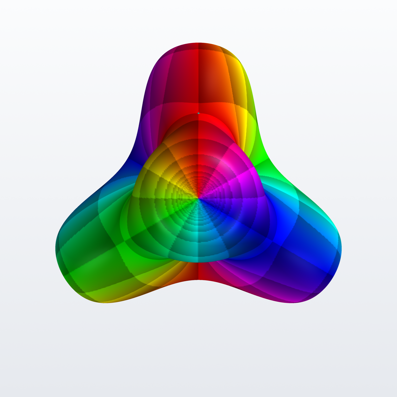
Four spikes on one tetrahedron over four pits on its antipode -- the two tetrahedra that together make the cube. Its symmetry is T (order 12, rotations only): alone in this family it has no mirror plane, so a cut through it gives two halves that are genuinely different rather than two copies of one part. That is the point of the piece.
Show the code
import complexplorer as cp
preset = cp.catalog.get("tetrahedral_dual")   # f(z) = (z**4 + 2j*sqrt(3)*z**2 + 1) / (z**4 - 2j*sqrt(3)*z**2 + 1)
cp.plot(preset.domain(), preset.func, cmap=preset.colormap())

# ---
import complexplorer as cp
preset = cp.catalog.get("tetrahedral_dual")   # f(z) = (z**4 + 2j*sqrt(3)*z**2 + 1) / (z**4 - 2j*sqrt(3)*z**2 + 1)
sc = preset.scaling()
cp.riemann_pv(preset.func, cmap=preset.colormap(),
              modulus_mode=sc["method"], modulus_params=sc["params"])  # relief