STL export and the physical workflow¶

The last step of the tour is an object you can hold. A Riemann relief — the modulus of a function displacing the surface of a sphere — is already a closed 3D shape, which is what makes it printable.

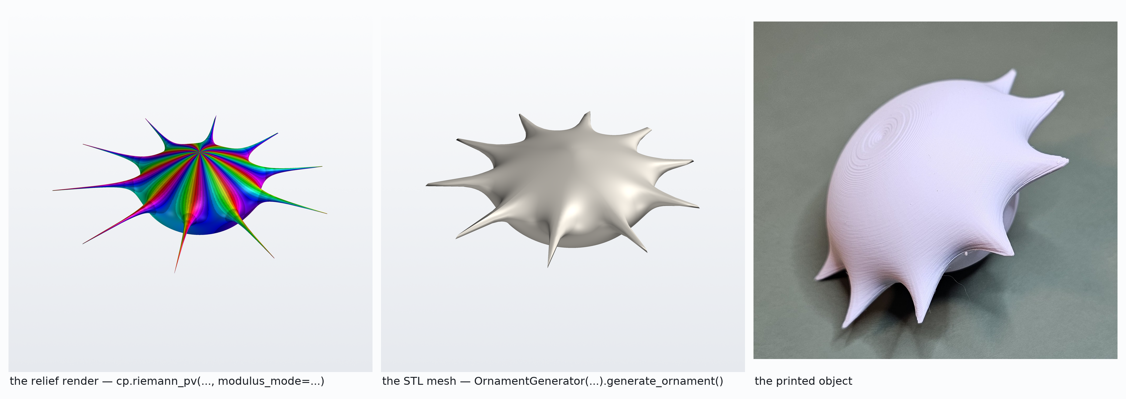
The relief is the mathematics, the mesh is the geometry that survives losing the colour, and the print is the object on a desk. Ten poles become ten spikes around the central zero.

One call¶

import complexplorer as cp

cp.create_ornament(lambda z: z / (z**10 - 1), "flower.stl", size_mm=80, resolution=200)

Or, when you want the generator around for more than one step:

from complexplorer.export.stl import OrnamentGenerator

ornament = OrnamentGenerator(lambda z: z / (z**10 - 1), resolution=200)
ornament.generate_and_save("flower.stl", size_mm=80)

From the command line:

complexplorer stl preset:pole_flower_10 --size-mm 80 --resolution 200 -o flower.stl

What the settings do¶

resolution is the sphere's sampling density, and it is the main quality dial. 150 is a reasonable default; 200–300 gives crisper spikes and a proportionally larger file.
normalize rescales |f| so that the arbitrary constant in front of your function stops changing the shape. On by default. See below — this is the setting that matters most.
pointiness sets how sharp the features are: the surface approaches a feature like distance ** (1 / pointiness), so 2.0 (the default) is sharper than a cone and 0.5 is a rounded dome.
contrast sculpts the body between the features, for pieces where the features alone leave it nearly spherical. Off by default.
scaling decides how |f(z)| becomes displacement. The default is logarithmic, a logistic curve in the log modulus, which is what pointiness tunes. scaling_params overrides anything derived from the parameters above.
size_mm is the printed size, applied at export, measured tip to tip — the object's true maximum width. Geometry is scaled at the end, so changing it does not change the shape. Pass size_measure="max" to size by the axis-aligned bounding box instead, as versions before 3.1 did.

Why is my ornament a blob¶

Nearly every ornament used to come out as "a sphere with features poked into it" regardless of the mathematics behind it. There were two causes, and they are worth understanding in this order, because the first carries most of the weight.

The scale of your function changes the shape¶

Every self-dual transfer puts sea level at |f| = 1. So f and 100 * f are not the same relief: multiplying by 100 raises the whole surface toward its ceiling, and the structure flattens against it. The constant in front of your function is arbitrary — it should change the labels, not the geometry.

Normalization fixes this by rescaling |f| so its area-weighted geometric mean over the sphere is exactly 1, which puts sea level in the middle of where the function actually lives:

# These now produce identical geometry. Before 3.1 they did not.
cp.create_ornament(lambda z: z / (z**10 - 1), "a.stl")
cp.create_ornament(lambda z: 100 * z / (z**10 - 1), "b.stl")

Measured on z / (z**10 - 1) at resolution=200, keeping everything else at the 3.0 defaults: normalizing moves the area-weighted share of the surface sitting in the middle half of the radial range — high means featureless — from 56.7% to 13.2%, a 4.3× improvement from one setting. For comparison, changing the transfer alone without normalizing moves the same number the wrong way, from 56.7% to 81.1%. Normalization is the fix; the transfer is a knob.

The geometric mean is the right average because it is self-dual: the constant for 1/f is the reciprocal of the constant for f, so the relief of 1/f is the relief of f turned inside out and nothing else changes. normalize="median" uses the area-weighted median instead, which holds up better when a high-order feature at infinity covers enough of the sphere to drag sea level away from the structure worth seeing. normalize=None switches it off, and a float sets the constant yourself.

If you know your function's complete divisor, cp.normalization_constant(zeros, poles, gain) gives the same constant in closed form. It is exact — but only for a complete divisor. Fed a partial list, or a transcendental function, it returns a confidently wrong number rather than an error: on the three commonly listed zeros of sin(z), which has infinitely many, it returns 0.092 against a true 0.853. This is also why the ornament path does not read divisors from a function preset's singularities field; those are illustrative, not complete. The default estimates the constant from the samples it already took, which has no such failure mode.

The transfer decides whether a tip is a cone or a dome¶

With r = r_min + delta * logistic(log|f| / k), the surface approaches a feature of order mu like distance ** (mu / k). The exponent mu / k — not k — is what the eye reads:

`mu / k`	what you see
greater than 1	a rounded dome, which reads as a blob
exactly 1	an exact cone
less than 1	a cusp, sharper than a cone

pointiness sets k = pointiness * pole_order, so the tip exponent is 1 / pointiness no matter what the function is. pole_order (default 1) is the order of the features you are shaping, and passing it means a double pole prints as sharp as a simple one instead of twice as blunt.

You have to tell the library the order; it does not guess. Fitting the scale to each function's log-modulus spread is the obvious move and a known dead end — it gives tip exponents anywhere from 1 to 8 and turns most pieces into rounded blobs, which is why the parameter is explicit.

The derived scale is capped at 6.0. Beyond roughly order 3 the mesh cannot deliver the dynamic range the rule assumes: a feature of order mu only drives log|f| as far as the nearest sample gets to it, so at order 5 an uncapped k = 10 wants log|f| to reach ±46 while a resolution-400 grid delivers about ±26 — and the body flattens instead of the tip sharpening. Measured on an order-5 icosahedral relief, the radial range used goes from 63% at k = 10 to 80% at k = 6. The cap is a no-op at order 3 and below, and it does not apply to sharpness, which you set deliberately.

The old arctan default could not express this. It has no scale at all: it reaches 90% of its height at |f| = 6.3 whatever your function does, which on a typical rational function is a tip exponent well above 1. That is the real reason the gallery pieces all looked related regardless of their mathematics.

The honest limit¶

A relief is only as interesting as its zero/pole divisor is dense. No amount of normalization or contrast changes that.

(z - 1) / (z + 1) is an egg at every setting, because |f| rises monotonically from one pole of the sphere to the other — there is one zero and one pole, they sit at opposite ends, and the surface in between has nothing to do but climb. A transfer function with three poles is the same story. If your piece is a smooth ovoid, check the divisor before reaching for another parameter: the answer is usually a function with more structure, not a better setting.

Sculpting the body with `contrast`¶

Raising pointiness sharpens the tips and squeezes everything else toward mid-radius; lowering it adds contrast across the body but blunts the tips. One parameter, two jobs, pulling opposite ways.

contrast=(boost, weight) breaks the tie by mixing two logistic curves: a narrow one at scale / boost carrying the bulk contrast, and the original wide one carrying the tips, weighted weight to 1 - weight.

# A few widely separated features, so the body would otherwise be a near-perfect sphere.
cp.create_ornament(lambda z: z / (z**4 - 1), "crown.stl", contrast=(3.0, 0.5))

Use it where a handful of features leave the body smooth; leave it off where the tips are the point of the piece. It is off by default for exactly that reason — applied globally it improves the pieces with sparse features and degrades the ones built around their spikes. In the ten-piece reference collection, six set it and four deliberately do not.

Measured at resolution=200 on the same area-weighted middle-half share as above, where lower means more sculpted. The middle column is the cost of sharper tips; the right-hand one is contrast paying most of it back:

function	3.0 defaults	3.1 defaults	3.1 + `contrast=(3.0, 0.5)`
`z / (z**4 - 1)`	59.6%	85.0%	65.4%
`z / (z**3 - 1)`	62.9%	90.0%	77.9%
`(z2 + 1) / (z2 - 1)`	81.6%	94.2%	84.2%
`z / (z**10 - 1)`	56.7%	23.3%	17.4%

The last row is the exception that shows the ordering of causes: that function's features are dense enough that normalization dominates, so the 3.1 defaults improve it outright and contrast only sharpens it further.

One honest caveat: asymptotically the wide term still sets the tip exponent, but that asymptote lies below mesh resolution, so in practice the tip climbs through only the last 1 - weight of the range and the visible point is shorter than the exponent implies.

Building a symmetric relief¶

The catalog carries six pieces whose reliefs have the full rotation symmetry of a Platonic solid:

import complexplorer as cp
from complexplorer.export.stl import OrnamentGenerator

star = cp.catalog.get("icosidodecahedral_star")
OrnamentGenerator.from_preset(star).generate_and_save("star.stl", size_mm=130)

from_preset matters here. These presets carry the relief settings their geometry needs — the star records pole_order=2 and resolution=400 — and rendering one without them gives the blunt, under-resolved version of the piece. cp.catalog.filter("polyhedral") returns the family.

Why these are ratios, and why the degrees must match¶

A rational map of degree d has exactly d zeros and d poles on the sphere, so a function with features at one solid's vertices and nowhere else does not exist. What does exist is a ratio of two relative invariants: each picks up an automorphy factor under a rotation, and the factors cancel only when the two forms have the same binary degree — at which point |f| descends to a genuinely invariant function.

So the star is H³/T², 60 over 60, where H is the icosahedral Hessian (roots: the 20 dodecahedron vertices) and T is the edge form (roots: the 30 edge midpoints). The eight forms are exported:

cp.tetrahedral_vertex, cp.tetrahedral_dual_vertex      # binary degree 4
cp.octahedral_vertex, cp.cube_vertex, cp.octahedral_edge     # 6, 8, 12
cp.icosahedral_vertex, cp.icosahedral_hessian, cp.icosahedral_edge   # 12, 20, 30

A ratio of unequal degree fails silently: it renders, it looks plausible, and it is not symmetric.

Watch for the forms that are one degree short as polynomials. cp.octahedral_vertex is binary degree 6 but degree 5, and cp.icosahedral_vertex is binary 12 but degree 11, because in each case one vertex sits at the north pole and projects to infinity. That missing root is a real spike or pit on the finished piece — four of the six presets have one — and it is invisible to anything that only reads the polynomial, including cp.normalization_constant, which takes finite divisors only.

Check the syzygy on any set you transcribe yourself¶

This is the part worth taking seriously. The forms quoted in the literature cohere as a set only for one particular orientation of the solid, and the commonly-remembered signs mix orientations. Pair z(z¹⁰ + 11z⁵ − 1) with the usual Hessian and you get three root sets that are each individually a perfect icosahedron, dodecahedron and edge set — while being rotated relative to one another. Every per-form geometry check passes. The ratios stop being rotation-invariant by a factor of 1e3 to 1e5.

Klein's syzygy is the check that catches it:

import numpy as np

z = np.array([0.3 + 0.7j, 1.4 - 0.2j])
left = cp.icosahedral_hessian(z)**3 - cp.icosahedral_edge(z)**2
right = 1728 * cp.icosahedral_vertex(z)**5
assert np.allclose(left, right)          # holds to ~1e-14 for the shipped forms

With the +11 variant that identity is wrong by a factor of about 20. cp.polyhedral_features(solid, kind) gives the projected feature locations the shipped coefficients were derived from, so you can check a form's roots directly as well.

Relief as a calibrated gain scale¶

sharpness sets the log-modulus scale directly, bypassing pointiness * pole_order. Setting it to ln(10) makes one unit of relief exactly one decade of gain — 20 dB — so walking a meridian reads off the Bode magnitude curve:

import numpy as np

H = cp.ee.TransferFunction([1], [1, 0.2, 1])
cp.create_ornament(H, "filter.stl", sharpness=float(np.log(10)))

That is not expressible as a tip exponent, which is why it is settable on its own. Conveniently ln(10) = 2.30 sits close to the default pointiness * 1 = 2.0, so a gain-calibrated piece still matches the sharpness of everything else.

A warning about `custom` scaling¶

A custom transfer must be smooth at |f| = 1, not merely monotone and odd.

A signed power of the log modulus — sign(L) * |L|**p — is monotone, odd about sea level, and very tempting. It also has infinite derivative at |f| = 1, which creases the surface along every sea-level contour and splits the mesh seam badly enough that the weld fails: the solid never closes and no repair will save it. This is recorded so the dead end is not walked a second time.

Your callable maps moduli into [0, 1], and the mode maps that onto [r_min, r_max]. Before 3.1 the bounds were silently discarded, so code written against that bug returns a radius directly — see the 3.1 migration note, because the fix changes such geometry without raising.

What happens before the file is written¶

generate_and_save repairs and checks the mesh, printing what it finds:

Repair (repair=True) cleans degenerate faces and closes small holes. Riemann sphere meshes are rectangular grids, so they have a seam along one meridian and a small cap missing at each pole; this is where those get welded and filled.
Normals are made consistent and outward-facing, so the facet normals recorded in the STL mean something to a slicer that reads them rather than recomputing.
Validation (validate=True) reports whether the mesh is watertight and manifold, its dimensions, its volume, and its minimum and maximum radius from the origin at the requested size.

The radii are the numbers to read, and they are measured before the mesh is centred — a relief is a star-shaped solid about the origin, so the body is at least 2 * min_radius_mm thick through the centre and there is no thin-wall failure mode to look for.

What the report does not measure is the ridge width between two adjacent pits, which is the thing that actually fails on a fused-deposition printer. min_radius_mm is the honest proxy for it, and the report says as much rather than substituting a number. Earlier versions printed an "estimated minimum wall thickness"; it was computed after scaling, evaluated to a constant False, and always recommended a size 2.67× larger. It is gone — see the 3.1 migration note if you were reading those keys.

Set verbose=False to silence the report, and validate=False to skip the checks if you are exporting in bulk and will inspect elsewhere.

What "size" means¶

size_mm is the object's true maximum width, measured tip to tip. That is a property of the shape. The obvious alternative — the largest dimension of the axis-aligned bounding box, which is what the library used before 3.1 — is a property of how the piece happens to sit in the coordinate frame:

from complexplorer.export.stl import max_extent

# A relief whose spikes point along the cube diagonals (+-1, +-1, +-1)/sqrt(3) projects each spike
# onto a coordinate axis at only 0.577 of its length, so its bounding box understates it by sqrt(3).

A collection sized by the box therefore comes out visibly uneven while every piece reports the same nominal size — the reference collection hit exactly this, with real extents running 80 to 137 mm at a nominal 80 mm and volumes spanning 13.7×, the largest object in the set being largest purely by accident of orientation.

max_extent() is the measure: the maximum support width over sampled directions, which for a convex body is the hull diameter. It samples Fibonacci directions plus the directions of the highest-radius points, because Fibonacci alone runs about 0.8% low when the widest direction is a spike axis it misses.

Pass size_measure="max" when the box is genuinely what you want — fitting a build plate, or reproducing a pre-3.1 export.

Printing notes¶

What comes out is a closed, roughly spherical shell with the function's poles as spikes. The spikes are the feature that fails: they are the thinnest part of the model and the furthest from the body, so they are where both slicing and printing go wrong first.

Two dials help, in this order:

Increase size_mm. Every feature scales with the model, so the ridges and tips that a nozzle cannot resolve at 30 mm usually clear it at 80 mm.
Blunt the tips. Lower pointiness for thicker, shorter spikes, and add contrast to keep the body interesting while you do — that pairing is what the parameter exists for.

Increasing resolution does not help here; it makes a finer mesh of the same thin geometry.

Orientation and supports are your slicer's business, and depend on the model and the printer. Complexplorer writes the geometry; it does not decide how it is printed.

Working with the mesh directly¶

from complexplorer.export.stl import validate_printability, scale_to_size, center_mesh

These operate on the PyVista PolyData, so a mesh can be checked, scaled and centred as part of a larger pipeline before it is written. max_extent measures true tip-to-tip width, and count_edges from the same module counts one class of edge at a time, which is less obvious than it sounds: PyVista's extract_feature_edges enables boundary, feature, manifold and non-manifold extraction all at once by default, so asking it for boundary edges alone reports every crease in a closed mesh as a hole.