Installation and your first portrait
Install
That is everything. PyVista is a required dependency as of 3.0, so 3D landscapes, Riemann spheres and STL export work out of the box — there is no optional 3D extra to remember and no capability flag to check. The install is large, mostly because VTK is; the backend policy records the measurement and the reasoning.
Optional extras:
pip install "complexplorer[qt]"       # interactive matplotlib windows in scripts
pip install "complexplorer[examples]" # tooling to run the example notebooks
Python 3.11 or newer is required.
Your first portrait
A portrait needs three things: a region of the plane, a function, and a colormap.
import complexplorer as cp

domain = cp.Rectangle(re_length=4, im_length=4)
func = lambda z: (z**2 - 1) / (z**2 + 1)
cmap = cp.Phase(phase_sectors=6, auto_scale_r=True)

cp.plot(domain, func, cmap=cmap, legend=True)
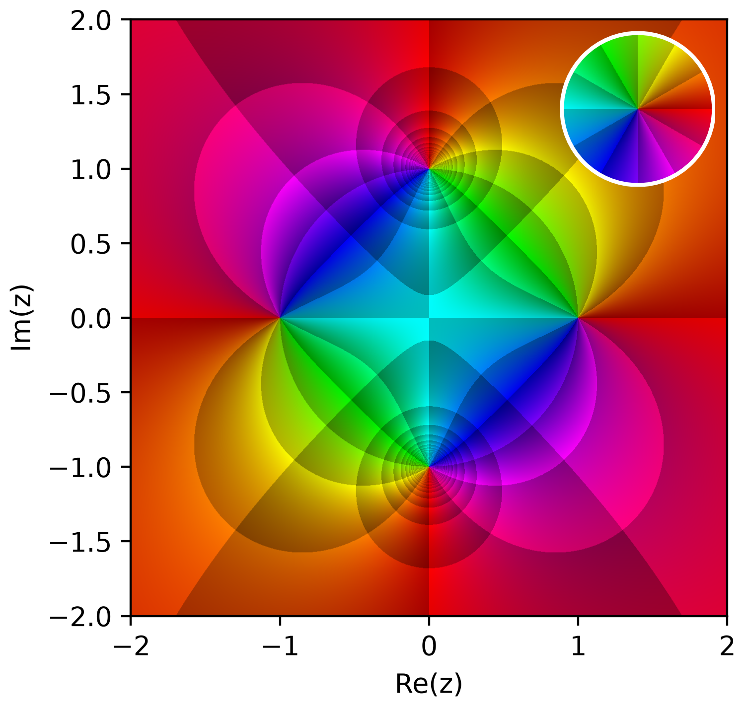
Four things are worth naming, because they recur everywhere in the library:
cmapis keyword-only in practice.plot(domain, func, cmap)will not do what you want; the third positional parameter isz, a pre-computed grid.phase_sectors=6cuts the colour wheel into six bands, so winding is countable rather than a smooth smear.auto_scale_r=Truesizes the modulus bands to match, which makes the cells square.legend=Trueinsets the same colormap applied to the identity map. It is the key to the picture: see reading a phase portrait.plotreturns the matplotlibAxes, so you can keep styling it.
Saving instead of showing
Every renderer takes filename, which writes the file instead of opening a window:
This is the form to use in scripts, in CI, and on a headless machine. The phase-wheel legend is drawn as an inset inside the portrait, not alongside it, so saving cannot crop it off.
Turning it into a landscape
The same domain, the same function, one different call:
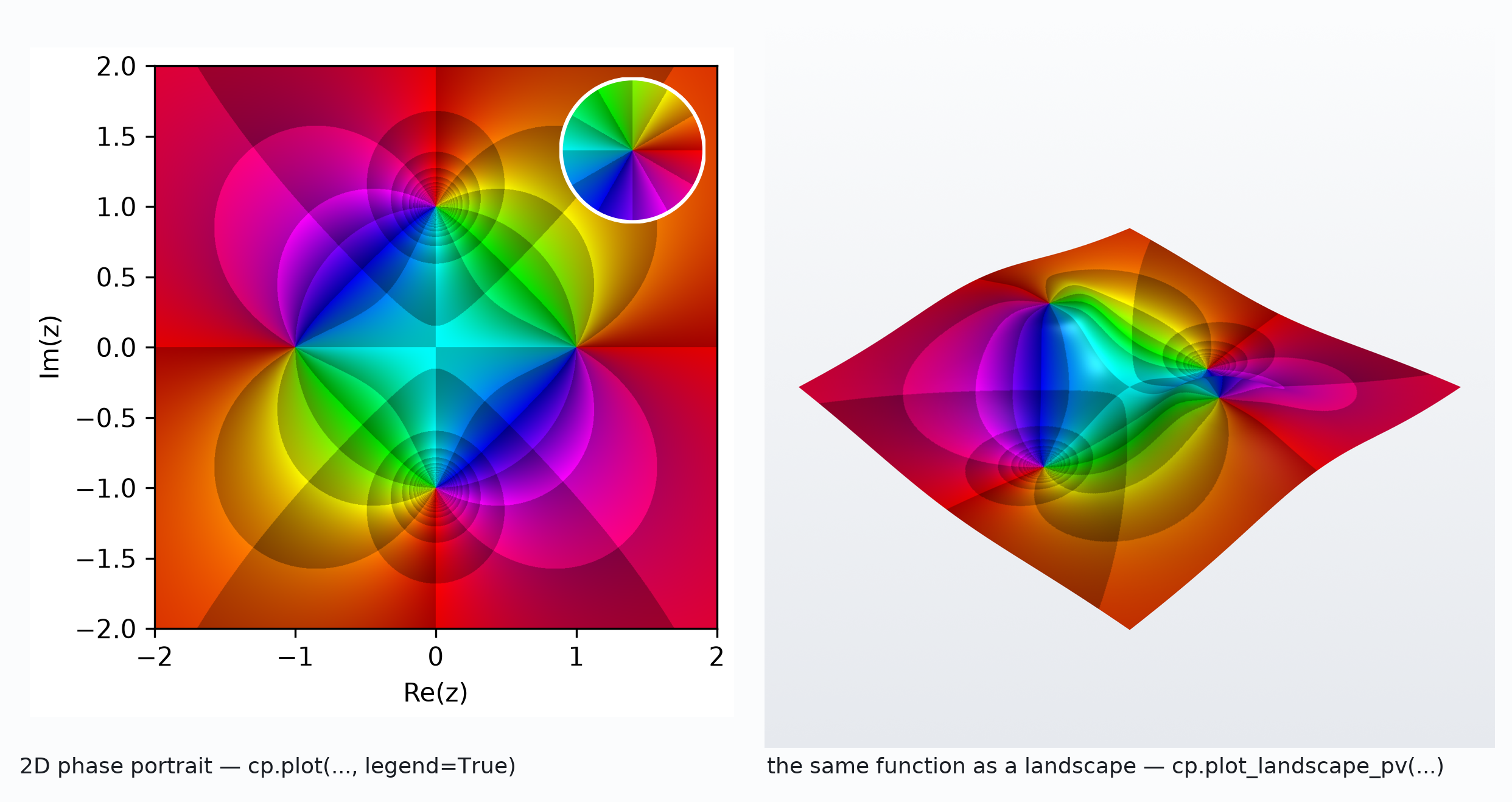
|f(z)| becomes height while the colours stay exactly as they were. That is the whole relationship
between the 2D and 3D views, and it is the subject of 3D landscapes and the Riemann
sphere.
One-liners
When you only want to look at something, quick_plot picks sensible defaults:
cp.quick_plot(lambda z: 1 / z)                  # 2D
cp.quick_plot(lambda z: 1 / z, mode="3d")       # analytic landscape
cp.quick_plot(lambda z: 1 / z, mode="riemann")  # Riemann sphere
Where to go next
- Reading a phase portrait — what the colours actually encode
- Domains and colormaps — regions you can do arithmetic on
- The gallery — every preset and colormap, with the code