Engineering mode

cp.ee aims the same machinery at linear systems. It is a namespace rather than a separate library: the objects it produces are ordinary callables that every renderer in complexplorer already accepts.

import complexplorer as cp

H = cp.ee.TransferFunction([1], [1, 0.2, 1])   # 1 / (s² + 0.2s + 1)
H.poles, H.zeros, H.is_stable

TransferFunction(num, den) takes coefficients in descending powers. system="z" switches to the discrete-time interpretation, where stability is about the unit circle rather than the left half-plane.

The four canonical views

cp.ee.transfer_portrait(H, legend=True)
cp.ee.pole_zero_plot(H)
cp.ee.bode_plot(H)
cp.ee.nyquist_plot(H)

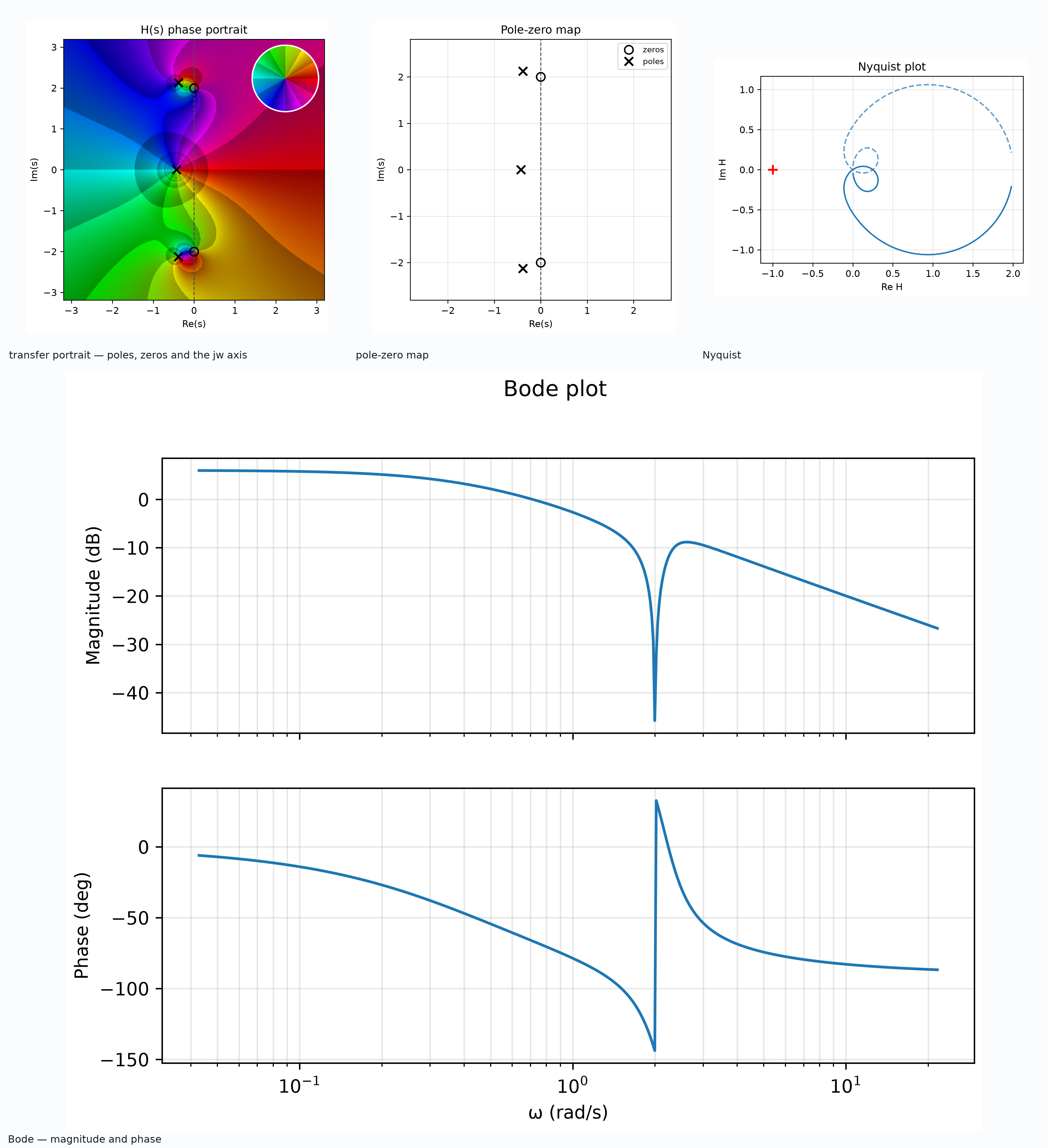
One stable transfer function in four views. The zeros sit exactly on the jω axis at ±2j — the notch — while the poles stay inside the left half-plane. The portrait shows where they are; Bode and Nyquist show what they do to a signal.

The transfer portrait is the piece the other three do not give you. A pole-zero map marks locations; the portrait colours the whole s-plane, so you see the field those poles and zeros create, with the jω axis drawn across it. Reading the colour along that axis is the frequency response: the portrait and the Bode plot are the same information, once as a map and once as a graph.

It is the same object throughout

cp.plot_landscape_pv(cp.Rectangle(6, 6), H)   # H is just a callable
cp.riemann_pv(H)

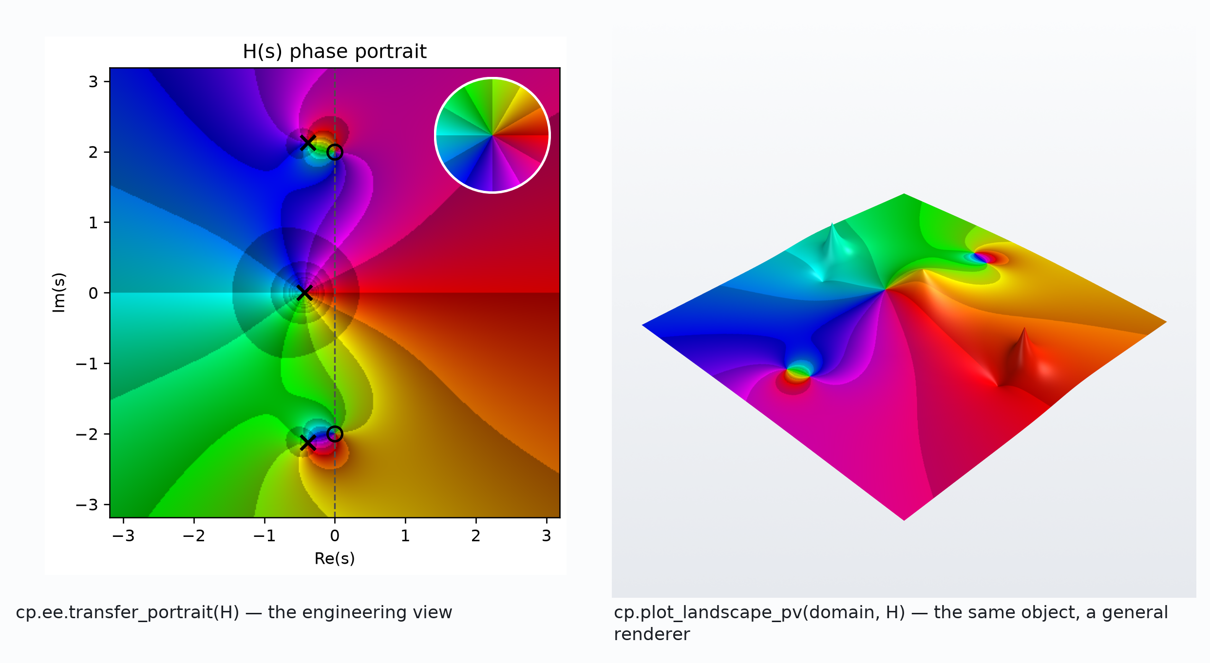
Nothing converts between the engineering view and the general one. The notch that reads as a dark point on the left is the valley on the right — the same function, drawn by two renderers.

This is worth knowing because it means everything else in the library applies: composite domains to cut out a pole, any colormap, filename for headless rendering, STL export if you want the thing on your desk.

Frequency response directly

omega, response = H.frequency_response()

is_stable is the quick check; poles and zeros are numpy arrays, so the usual analysis is a line away.